
All Solutions
Page 738: Assessment
In contrast, charging by contact involves an actual transfer of charges between the charging source and the object to charge. Moreover, the charged object acquires a charge with the same sign as the charge on the charging source.
$$
E = frac{F}{|q|} = frac{0.80;mathrm{N}}{3.6times10^{-6};mathrm{C}} = 2.2times10^5;mathrm{N/C}
$$
$$
|q| = frac{F}{E} = frac{0.61;mathrm{N}}{4.7times10^4;mathrm{N/C}} = 13;mumathrm{C}
$$
We see the charge on the object is $-13;mu$C.
$$
F = ma
$$
where $F$ is the electric force. We express $F$ as $F = |q|E$ and solve for $E$:
$$
begin{align*}
|q|E &= ma\
E &= frac{ma}{|q|}
end{align*}
$$
Substituting the known values, we find
$$
begin{align*}
E &= frac{(0.017;mathrm{kg})(3.3;mathrm{m/s}^2)}{5.6times10^{-6};mathrm{C}}\
&= 1.0times10^4;mathrm{N/C}
end{align*}
$$
$textbf{(b)}$ The magnitude of the electric field can be calculated using $E=kq/r^2$, with $r = 0.45$ m:
$$
begin{align*}
E &= kfrac{q}{r^2}\
&= (8.99times10^9;mathrm{N}cdotmathrm{m^2}/mathrm{C^2})timesfrac{5.7times10^{-6};mathrm{C}}{(0.45;mathrm{m})^2}\
&= 2.5times10^5;mathrm{N/C}
end{align*}
$$
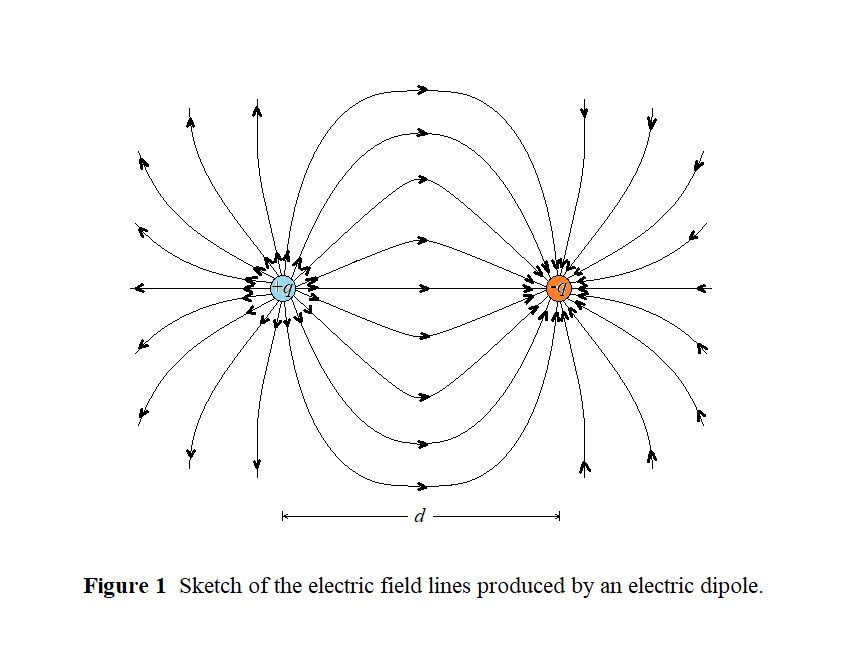
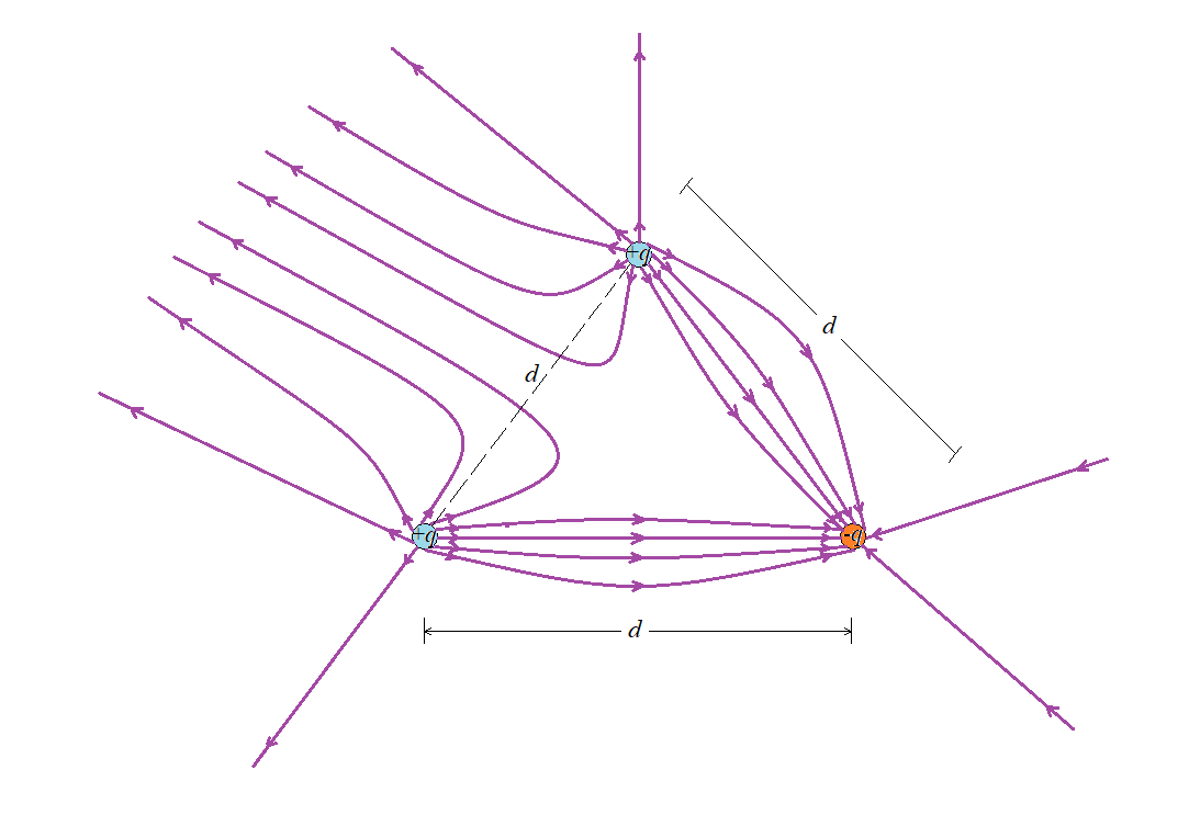
$textbf{(b)}$ We see from Figure 20.26 that all the field lines starting from the positive charges $q_1$ and $q_3$ end at the negative charge $q_2$. It follows that the magnitudes of the three charges are related by $|q_1| + |q_3| = |q_2|$. By symmetry (the situation in Figure 20.26 is symmetric about a vertical line passes through $q_2$), $q_1$ and $q_3$ must have the same magnitude. Accordingly, we have
$$
begin{align*}
2|q_1| &= |q_2|\
|q_1| &= frac{|q_2|}{2} = frac{10.0;mumathrm{C}}{2} = 5.00;mumathrm{C}
end{align*}
$$
That we have $q_1 = +5.00;mu$C.
$textbf{(c)}$ It also follows, by symmetry, that $q_3 = q_1 = +5.00;mu$C.
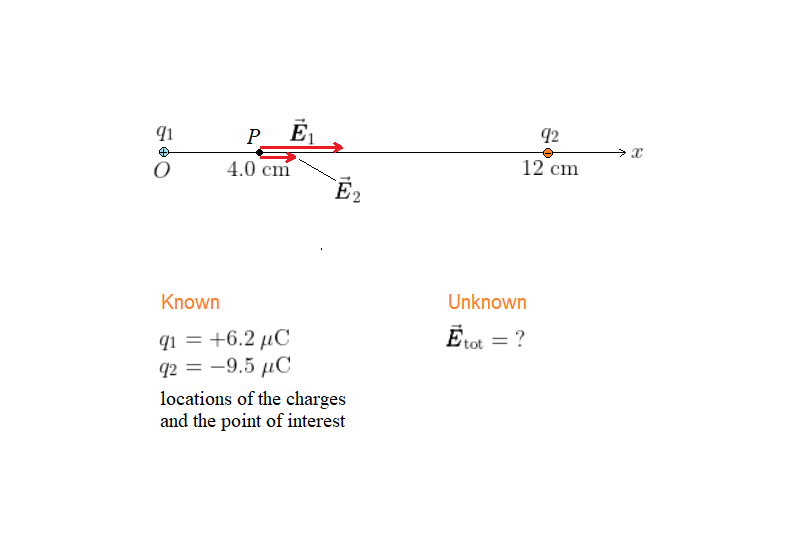
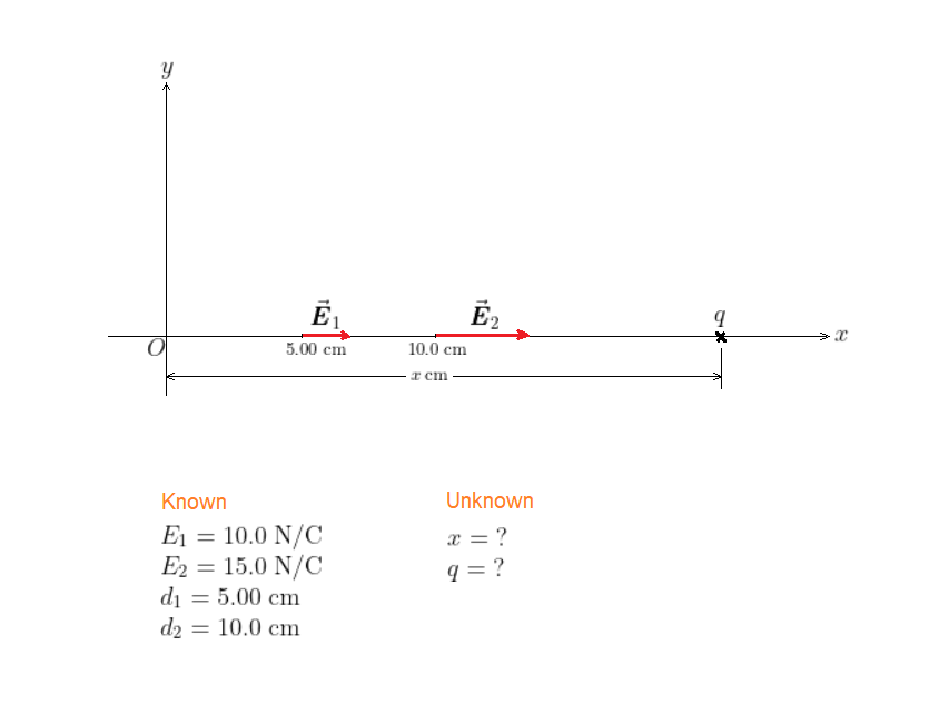
The situation is shown in our sketch, with each charge and the point $P$ (of interest) at its appropriate positions. We also show the electric field produced by each charge. Notice that at $P$ the electric fields due to the individual charges point in the positive $x$ direction; so we expect the total electric field to point in the positive $x$ direction.
$text{color{#4257b2}Strategy}$
The total electric field at $P$ is the vector sum of the electric fields produced by $q_1$ and $q_2$. In particular, notice that $vec{pmb E}_1$ and $vec{pmb E}_2$ add in the same direction. The magnitude of $vec{pmb E}_1$ is $k|q_1|/r^2$, with $r = 4.0$ cm. Similarly, the magnitude of $vec{pmb E}_2$ is $k|q_2|/r^2$, with $r = 8.0$ cm.
$text{color{#4257b2}Solution}$
The electric field produced by $q_1$ at $P$ is
$$
begin{align*}
vec{pmb E}_1 &= kfrac{q_1}{r^2}\
&= (8.99times10^9;mathrm{N}cdotmathrm{m}^2/mathrm{C}^2)frac{(6.2times10^{-6};mathrm{C})}{(4.0times10^{-2};mathrm{m})^2}\
&= 3.5times10^7;mathrm{N/C}qquad(text{positive};x;text{direction})
end{align*}
$$
The electric field produced by $q_2$ at $P$ is
$$
begin{align*}
vec{pmb E}_2 &= kfrac{q_2}{r^2}\
&= (8.99times10^9;mathrm{N}cdotmathrm{m}^2/mathrm{C}^2)frac{(9.5times10^{-6};mathrm{C})}{(8.0times10^{-2};mathrm{m})^2}\
&= 1.3times10^7;mathrm{N/C}qquad(text{positive};x;text{direction})
end{align*}
$$
We then add these two electric fields to find the total electric field, $vec{pmb E}_{rm tot}$, at $P$:
$$
begin{align*}
vec{pmb E}_{rm tot} &= vec{pmb E}_1 + vec{pmb E}_2\
&= 3.5times10^7;mathrm{N/C} + 1.3times10^7;mathrm{N/C}\
&= 4.8times10^7;mathrm{N/C}qquad(text{positive};x;text{direction})
end{align*}
$$
$text{color{#4257b2}Insight}$
The total electric field at $P$ has a magnitude of $4.8times10^7$ N/C, and it points in the positive $x$ direction. Notice that the electric field produced by $q_1$ is greater than that produced by $q_2$, even though $q_2$ has the greater magnitude. The reason is that $q_1$ is three times closer to $P$ than $q_2$ is.
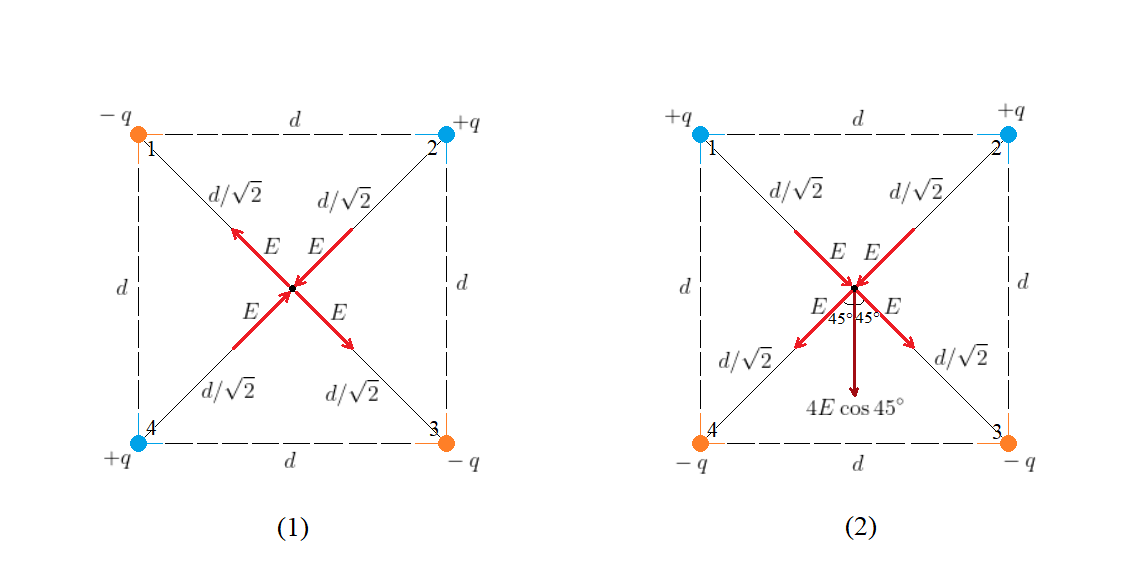
$textbf{(b)}$ The magnitude of the electric field produced by each charge on the corners of the square at the center of the square is $E = kq/r^2$, with $r = d/sqrt{2}$.
For case (1), we’ve seen how the electric fields due to the individual charges cancel each other in pairs [see Fig. (1)], leading to zero total electric field at the center of the square.
For case (2), the total electric field at the center of the square point downward [see Fig. (2)] with a magnitude of
$$
4Ecos45^circ = 4kfrac{q}{(d/sqrt{2})^2}cdotfrac{1}{sqrt{2}} = 4sqrt{2};frac{kq}{d^2}
$$
$$
E_1 = kfrac{|q|}{(x – 5.00;{rm cm})^2}
$$
Similarly, the magnitude of the electric field at $x = 10.0$ cm is
$$
E_2 = kfrac{|q|}{(x – 10.0;{rm cm})^2}
$$
Dividing $E_2$ by $E_1$ and using the known values of $E_1$ and $E_2$, we have
$$
frac{15.0;{rm N/C}}{10.0;{rm N/C}} = frac{(x – 5.00;{rm cm})^2}{(x – 10.0;{rm cm})^2}
$$
We simplify the result and obtain the following quadratic equation in $x$:
$$
x^2 – (40.0;{rm cm})x + 250;{rm cm}^2 = 0
$$
which has the solutions $x = 32.2$ cm and $x = 7.75$ cm. The latter is not accepted, as it doesn’t satisfy $x > 10.0$ cm, so the correct location of the point charge should be $x = 32.2$ cm.
$$
begin{align*}
E_1 &= kfrac{|q|}{(32.2;{rm cm} – 5.00;{rm cm})^2}\
|q| &= frac{(27.2;{rm cm})^2E_1}{k}\
|q| &= frac{(27.2times10^{-2};{rm m})^2(10.0;{rm N/C})}{8.99times10^9;mathrm{N}cdotmathrm{m}^2/mathrm{C}^2}\
&= 82.3;mumathrm{C}
end{align*}
$$
We see the point charge is $q = -82.3;mu$C.
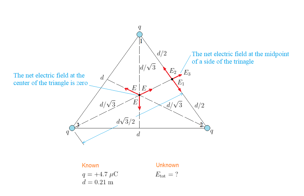
$textbf{(a)}$ As shown in our sketch, at the midpoint of (the right) side of the triangle the electric fields produced by charges 1 and 2 have the same magnitude $(E_1 = E_2)$ and opposite directions, leading to a complete cancelation. As a result, the total electric field is only due to the (uncanceled) electric field produced by charge 3. In such case, the magnitude of the electric field due to charge 3 at the required position is $E_3 = kq/r^2$, with $r = dsqrt{3}/2$, and thus the magnitude of the net electric field is
$$
begin{align*}
E_{rm tot} = E_3 &= kfrac{q}{(dsqrt{3}/2)^2}\
&= kfrac{4q}{3d^2}\
&= (8.99times10^9;mathrm{N}cdotmathrm{m}^2/mathrm{C}^2)timesfrac{4times(4.7times10^{-6};mathrm{C})}{3times(0.21;mathrm{m})^2}\
&= 1.3times10^6;mathrm{N/C}
end{align*}
$$
By symmetry, this is the same magnitude of the electric field at the midpoint of any of the three sides of the triangle (rotate the whole sketch $60^circ$ in either direction and the same result will be obtained).
$textbf{(b)}$ Referring to our sketch again, we can see at the center of the triangle the electric fields produced by the individual charges have the same magnitude and, moreover, are arranged in a three-fold symmetric configuration (the three electric fields are oriented such that the mutual angle between any two of them is exactly $60^circ$). The result is a zero net electric field at the center of the triangle (note that the three vectors can be arranged to form a complete triangle, leading to zero vector sum).
In such case, we can see the magnitude of the electric field at the center of the triangle is less than that at the midpoint of a side.
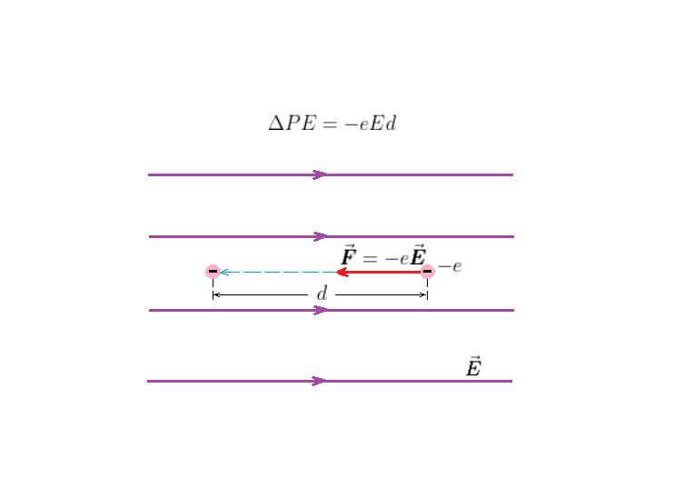
$$
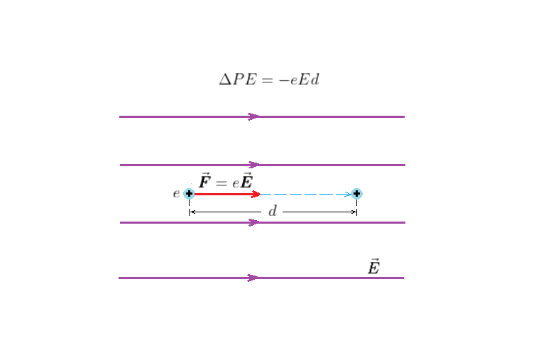
W = eEd
$$
The equation from Chapter 6 that relates work and potential energy, $Delta PE = -W$, gives a direct connection between the work done to move charges in an electric field and the system’s change in electric potential energy:
$$
Delta PE = -Wqquadtext{or}qquad Delta PE = -eEd
$$
We see the electric potential energy of the system $decreases$ in this case.
$textbf{(b)}$ The $best$ explanation is the choice $textbf{B.}$
As the electron begins to move, its kinetic energy increases. The increase in kinetic energy is equal to the decrease in the electric potential energy of the system.
In such case, the arrangements A and B correspond to zero total charge each. The arrangement C corresponds to a total charge of $-3q$. The final arrangement D corresponds to a total charge of $+q$. Hence, the rank for the four arrangements in order of increasing electric potential at the origin goes like $rm C < A = B < D$.
rm C < A = B < D
$$
The equation $E = -Delta V/d$ gives us a direction connection between the electric field and the change in the electric potential, from which we can determine the magnitude of the electric field. It also tells us the electric potential decreases in the direction of the electric field.
$text{color{#4257b2}Solution}$
Substitute $d = 0.10;mu$m and $Delta V = -0.070$ V in $|E| = |Delta V|/d$:
$$
|E| = frac{|Delta V|}{d} = frac{0.070;mathrm{V}}{0.10times10^{-6};mathrm{m}} = 7.0times10^5;mathrm{V/m}
$$
Since the electric potential inside the living cell is lower than that outside, then the electric field must point from the outside inward and through the cell membrane toward inside of the cell.
$$
begin{align*}
frac{1}{2}m_pv_2^2 &= frac{1}{2}m_pv_1^2 + PE_1 – PE_2\
&= frac{1}{2}m_pv_1^2 + e(V_1 – V_2)
end{align*}
$$
Next we set $v_1 = 0$, since the particle starts at rest, and solve for $v_2$:
$$
begin{align*}
frac{1}{2}m_pv_2^2 &= e(V_1 – V_2)\
v_2 &= sqrt{frac{2e(V_1 – V_2)}{m_p}}
end{align*}
$$
Realizing that the proton has a charge of magnitude $e = 1.60times10^{-19}$ C and a mass of $m_p = 1.67times10^{-27}$ kg and substituting the other known values, we find
$$
begin{align*}
v_2 &= sqrt{frac{2(1.60times10^{-19};mathrm{C})(275;mathrm{V})}{(1.67times10^{-27};mathrm{kg})}}\
&= 2.30times10^5;mathrm{m/s}
end{align*}
$$
As the object begins to move, its kinetic energy increases. The gained kinetic energy $Delta KE$ is equal to the decrease in the electric potential energy $Delta PE$ of the system. The equation $Delta PE = qDelta V$ gives us a direct connection between the change in the electric potential energy and the corresponding potential difference, from which we can determine the value of $Delta V$.
$text{color{#4257b2}Solution}$
The gained kinetic energy is equal to the change in the electric potential energy:
$$
Delta KE = Delta PE = qDelta V
$$
Solve for $Delta V$ and substitute $Delta KE = 0.0014$ J and $q = 3.1;mu$C:
$$
begin{align*}
Delta V &= frac{Delta KE}{q}\
&= frac{(0.0014;mathrm{J})}{(3.1times10^{-6};mathrm{C})}\
&= 450;mathrm{V}
end{align*}
$$
$$
begin{align*}
frac{1}{2}m_ev_2^2 &= frac{1}{2}m_ev_1^2 + PE_1 – PE_2\
&= frac{1}{2}m_ev_1^2 + (-e)(V_1 – V_2)
end{align*}
$$
Next we set $v_1 = 0$ (as the electrons are accelerated from rest) and solve for $v_2$:
$$
begin{align*}
frac{1}{2}m_ev_2^2 &= e(V_2 – V_1)\
v_2 &= sqrt{frac{2e(V_2 – V_1)}{m_e}}
end{align*}
$$
We realize the electrons have a charge of magnitude $e = 1.6times10^{-19}$ C and a mass of $m_e = 9.1times10^{-31}$ kg and substitute the other know values:
$$
begin{align*}
v_2 = &= sqrt{frac{2(1.6times10^{-19};mathrm{C})(25times10^3;mathrm{V})}{9.1times10^{-31};mathrm{kg}}}\
&= 9.4times10^7;mathrm{m/s}
end{align*}
$$
$$
begin{aligned}
V = k frac{q}{r}
end{aligned}
$$
where $k = 8.99times 10^{9};text{N}cdot text{m}^2/text{C}^2$ is the Coulomb constant, $q$ is the charge, and $r$ is the distance from the charge.
**Given**
Charge of a proton: $e = 1.6times 10^{-19};text{C}$
Radial distance between the proton and the electron’s orbit: $r = 0.529times 10^{-10};text{m}$
$$
begin{aligned}
V &= (8.99times 10^{9};text{N}cdot text{m}^2/text{C}^2) left(frac{1.6times 10^{-19};text{C}}{0.529times 10^{-10};text{m}}right) \ &= boxed{27.2;text{V}}
end{aligned}
$$
$textbf{(a)}$ The equation $E = -Delta V/d$ gives us a direct connection between the electric field and the corresponding electric potential, which can be used to solve for the value of $Delta V$. $textbf{(b)}$ It also tells us that if the separation $d$ is increased, the required potential difference $Delta V$ (to obtain the same $E$) increases.
$text{color{#4257b2}Solution}$
$textbf{(a)}$ Substitute $E = 3.0times10^6$ V/m and $d = 0.0635$ cm into $Delta V = -Ed$:
$$
Delta V = -(3.0times10^6;mathrm{V/m})(0.0635times10^{-2};mathrm{m}) = -1.9;mathrm{kV}
$$
$textbf{(b)}$ From the relationship $|Delta V| = Ed$, we can infer that the potential difference, required for the same value of $E$, increases as the separation $d$ of the electrodes is increased.
$$
begin{aligned}
E = frac{1}{2}QV
end{aligned}
$$
where $Q$ is the battery’s charge and $V$ is the voltage.
The kinetic energy is calculated using the formula:
$$
begin{aligned}
text{KE} = frac{1}{2}mv^2
end{aligned}
$$
**GIVEN**
Voltage: $V = 12;text{V}$
Charge: $Q = 7.5times 10^{5};text{C}$
Mass: $m = 1400;text{kg}$
$$
begin{aligned}
E = frac{1}{2}(7.5times 10^{5};text{C})(12;text{V}) = 4.5times 10^{6};text{J}
end{aligned}
$$
$$
begin{aligned}
v &= sqrt{frac{2text{KE}}{m}} \ &= sqrt{frac{2(4.5times 10^{6};text{J})}{1400;text{kg}}} \ &= boxed{80;text{m/s}}
end{aligned}
$$
As the proton slows down its speed to rest, its kinetic energy decreases. The lost kinetic energy $Delta KE$ is equal to the increase in the electric potential energy $Delta PE$ of the system. The kinetic energy of the proton is equal to $m_pv^2/2$ ($m_p$ is the proton’s mass) and the equation $Delta PE = qDelta V$ (with $q = e$ for the proton) gives us a direct connection between the electric potential energy and the corresponding potential difference, from which we can find the value of $Delta V$.
$text{color{#4257b2}Solution}$
The conversion of energy gives us:
$$
Delta KE = Delta PE
$$
which leads to
$$
frac{1}{2}m_pv^2 = eDelta V
$$
Solve for $Delta V$ and substitute the known values ($e = 1.60times10^{-19}$ C and $m_p = 1.67times10^{-27}$ kg for the proton):
$$
begin{align*}
Delta V &= frac{m_pv^2}{2e}\
&= frac{(1.67times10^{-27};mathrm{kg})(4.0times10^5;mathrm{m/s})^2}{2(1.6times10^{-19};mathrm{C})}\
&= 840;mathrm{V}
end{align*}
$$
$$
begin{aligned}
Delta V= V_text{B}-V_text{A}=boxed{0}
end{aligned}
$$
$$
begin{aligned}
Delta V =-Ed
end{aligned}
$$
where $E$ is the magnitude of the electric field and $d$ is the distance.
$$
begin{aligned}
Delta V =-(1200frac{text{N}}{text{C}})(0.04;text{m})=-48frac{text{N}cdottext{m}}{text{C}}=boxed{-48;text{V}}
end{aligned}
$$
The total electric potential due to multiple charges is equal to the algebraic sum of the potentials due to the individual charges. Therefore, the electric potential at point P, in Fig. 20.30, is the algebraic sum of the potentials due to the given three charges on the vertices of the triangle. In particular, the electric potential due to the $+2.75$-$mu$C charge at P is equal to $V_1 = kq/r$, with $q = +2.75;mu$C and $r = 0.625$ m. Similarly, the electric potential due to the $-1.72$-$mu$C charge at P is equal to $V_2 = kq/r$, with $q = -1.72;mu$C and $r = 0.625$ m. Finally, from the geometry of Fig. 20.30 the separation between the leftover charge (of $+7.45;mu$C) and P is equal to $(1.25;mathrm{m})sqrt{3}/2 = 1.08$ m, so the electric potential due to the $+7.45$-$mu$C charge at P is equal to $V_3 = kq/r$, with $q = +7.45;mu$C and $r = 1.08$ m.
$text{color{#4257b2}Solution}$
The electric potential due to the $+2.75$-$mu$C charge at P is
$$
begin{align*}
V_1 &= (8.99times10^9;mathrm{N}cdotmathrm{m}^2/mathrm{C}^2)timesfrac{(+2.75times10^{-6};mathrm{C})}{(0.625;mathrm{m})}\
&= 4.0times10^4;mathrm{V}
end{align*}
$$
The electric potential due to the $+2.75$-$mu$C charge at P is
$$
begin{align*}
V_2 &= (8.99times10^9;mathrm{N}cdotmathrm{m}^2/mathrm{C}^2)timesfrac{(-1.72times10^{-6};mathrm{C})}{(0.625;mathrm{m})}\
&= -2.5times10^4;mathrm{V}
end{align*}
$$
The electric potential due to the $+7.45$-$mu$C charge at P is
$$
begin{align*}
V_3 &= (8.99times10^9;mathrm{N}cdotmathrm{m}^2/mathrm{C}^2)timesfrac{(+7.45times10^{-6};mathrm{C})}{(1.08;mathrm{m})}\
&= 6.20times10^4;mathrm{V}
end{align*}
$$
Hence, the electric potential at P is
$$
begin{align*}
V &= V_1 + V_2 + V_3\
&= (4.0times10^4;mathrm{V}) + (-2.5times10^4;mathrm{V}) + (6.20times10^4;mathrm{V})\
&= 7.7times10^4;mathrm{V}
end{align*}
$$
The total electric potential due to multiple charges is equal to the algebraic sum of the potentials due to the individual charges. Let us call the point at the empty corner of the rectangle P. The electric potential at point P (see Fig. 20.31) is the algebraic sum of the potentials due to the given three charges on the corners of the rectangle. In particular, the electric potential at P due to the $-3.3$-$mu$C charge is equal to $V_1 = kq/r$, with $q = -3.3;mu$C and $r = 0.25$ m. From the geometry of Fig. 20.31 the separation between the upper-left charge (of $-6.1;mu$C) and P is equal to 0.30 m, so the electric potential at P due to the $-6.1$-$mu$C charge is equal to $V_2 = kq/r$, with $q = -6.1;mu$C and $r = 0.30$ m. Finally, the electric potential at P due to the $+2.7$-$mu$C charge is equal to $V_3 = kq/r$, with $q = +2.7;mu$C and $r = 0.16$ m.
$text{color{#4257b2}Solution}$
The electric potential at P due to the lower-left charge is
$$
begin{align*}
V_1 &= (8.99times10^9;mathrm{N}cdotmathrm{m}^2/mathrm{C}^2)timesfrac{(-3.3times10^{-6};mathrm{C})}{(0.25;mathrm{m})}\
&= -1.2times10^5;mathrm{V}
end{align*}
$$
The electric potential at P due to the upper-left charge is
$$
begin{align*}
V_2 &= (8.99times10^9;mathrm{N}cdotmathrm{m}^2/mathrm{C}^2)timesfrac{(-6.1times10^{-6};mathrm{C})}{(0.30;mathrm{m})}\
&= -1.8times10^5;mathrm{V}
end{align*}
$$
The electric potential at P due to the upper-right charge is
$$
begin{align*}
V_3 &= (8.99times10^9;mathrm{N}cdotmathrm{m}^2/mathrm{C}^2)timesfrac{(+2.7times10^{-6};mathrm{C})}{(0.16;mathrm{m})}\
&= 1.5times10^5;mathrm{V}
end{align*}
$$
Hence, the electric potential at P is
$$
begin{align*}
V &= V_1 + V_2 + V_3\
&= (-1.2times10^5;mathrm{V}) + (-1.8times10^5;mathrm{V}) + (1.5times10^5;mathrm{V})\
&= -1.5times10^5;mathrm{V}
end{align*}
$$
$textbf{(a)}$ The equation $E = -Delta V/d$ gives us a direct connection between the electric field and the corresponding electric potential. The geometric interpr-
etation of this relationship is that the magnitude of the electric field is given by how much steep the graph of the electric potential versus the position. That the region within which the $V$-$x$ graph (shown in Fig. 20.32) is steep the most is the one with the electric field of the greatest magnitude. $textbf{(b)}$ Using the $V$-$x$ graph shown in Fig. 20.32, we can divide the change in the electric potential $Delta V$ by the corresponding distance $d = Delta x$, to calculate the magnitude of the electric field in each region.
$text{color{#4257b2}Solution}$
$textbf{(a)}$ By inspection, we see region 4 corresponds to the steepest $V$-$x$ line. In such case, the electric field has the greatest magnitude in region 4.
$textbf{(b)}$ In region 1, we have $Delta V = (6.0 – 8.0)$ V = $-2.0$ V and $d = Delta x = (0.15 – 0)$ m = 0.15 m. Thus the electric field in this region has the magnitude
$$
E = -frac{Delta V}{d} = -frac{(-2.0;mathrm{V})}{(0.15;mathrm{m})} = 13;mathrm{V/m}
$$
In region 2, the value of $V$ is constant with $x$; that is, $Delta V = 0$. In such case, the electric field in this region is identically zero.
In region 3, we have $Delta V = (8.0 – 6.0)$ V = $2.0$ V and $d = Delta x = (0.60 – 0.25)$ m = 0.35 m. Thus the electric field in this region has the magnitude
$$
E = frac{Delta V}{d} = frac{(2.0;mathrm{V})}{(0.35;mathrm{m})} = 5.7;mathrm{V/m}
$$
Finally, in region 4 we have $Delta V = (1.0 – 8.0)$ V = $-7.0$ V and $d = Delta x = (0.70 – 0.60)$ m = 0.10 m. Thus the electric field in this region has the magnitude
$$
E = -frac{Delta V}{d} = -frac{(-7.0;mathrm{V})}{(0.10;mathrm{m})} = 70;mathrm{V/m}
$$
$text{color{#4257b2}Insight}$
As we can see from the results in part (b), the electric field has the greatest magnitude (of 70 V/m) in region 4, which corresponds to the steepest part of the $V$-$x$ graph.
$$
begin{aligned}
C=frac{Q}{V}
end{aligned}
$$
wherein $Q$ is the magnitude of the charge in either plate and $V$ is the magnitude of the voltage difference between its plates.
$$
begin{aligned}
C=frac{Q}{V}
end{aligned}
$$
wherein $Q$ is the magnitude of charge on either plate and $V$ is the electric potential difference.
$$
begin{aligned}
Q&=CV\&=(4.1times10^{-6};text{F})(12;text{V})\&=boxed{49.2;mutext{C}}
end{aligned}
$$
$$
begin{aligned}
V=frac{Q}{C}
end{aligned}
$$
$$
begin{aligned}
V&=frac{8.2times10^{-9};text{C}}{320times10^{-12};text{F}}\&=boxed{25.6;text{V}}
end{aligned}
$$
$$
begin{aligned}
C=frac{Q}{V}
end{aligned}
$$
wherein $Q$ is the magnitude of charge on either plate and $V$ is the electric potential difference.
$$
begin{aligned}
C&=frac{6.9times10^{-9};text{C}}{1.5;text{V}}\&=boxed{4.6;text{nF}}
end{aligned}
$$
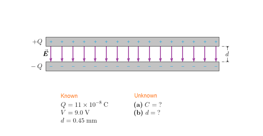
The capacitor is shown in our sketch. Notice that the charge on each plate has the magnitude $Q$. The electric field is uniform and points from the positive plate to the negative plate.
$text{color{#4257b2}Strategy}$
$textbf{(a)}$ Capacitance is defined as $C = Q/V$. We can use this expression to find the capacitance of our capacitor; the charge and the voltage are given in the problem statement. $textbf{(b)}$ In Lesson 20.2 we saw that the electric field is $E = -Delta V/d$. It follows that the magnitude of the electric field is $|E| = |Delta V|/d$. The voltage difference, $Delta V$, is the battery voltage $V$ given in the problem statement. The distance $d$ is the distance between the plates. Therefore, $d = 0.45$ mm.
$text{color{#4257b2}Solution}$
$textbf{(a)}$ Use $C = Q/V$ to find capacitance of the capacitor:
$$
C = frac{Q}{V} = frac{1.1times10^{-8};mathrm{C}}{9.0;mathrm{V}} = 1.2;mathrm{nF}
$$
$textbf{(b)}$ The magnitude of the electric field between the plates is $|E| = |Delta V|/d$, with $d = 0.45$ mm = $0.45times10^{-3}$ m:
$$
|E| = frac{|Delta V|}{d} = frac{9.0;mathrm{V}}{0.45times10^{-3};mathrm{m}} = 2.0times10^4;mathrm{V/m}
$$
$$
begin{aligned}
V=frac{Q}{C}=lvert E rvert d
end{aligned}
$$
where $Q$ is the magnitude of the charge on either plate, $C$ is the capacitance of the capacitor, $lvert E rvert$ is the magnitude of the electric field and $d$ is the plate separation.
$$
begin{aligned}
C=frac{Q}{lvert E rvert d}
end{aligned}
$$
$$
begin{aligned}
C&=frac{6.7times10^{-9};text{C}}{29000frac{text{V}}{text{m}} (0.35times10^{-3};text{m})}\&=boxed{660.1;text{pF}}
end{aligned}
$$
$textbf{(a)}$ The energy stored in the capacitor is given by $PE = frac{1}{2}QV$. Using the definition of the capacitance $C = Q/V$, we have $Q = CV$ and so $PE = frac{1}{2}CV^2$. As the motor lifts the mass, the energy in the capacitor is converted to a gravitational potential energy of magnitude $mtextit{g}h$, with $m = 5.0$ g and $h$ being the height to which the mass is lifted. We can solve the equation $frac{1}{2}CV^2 = mtextit{g}h$ for $h$ to find its value. $textbf{(b)}$ This time we apply the procedure in part (a) backwards. That we use the expression for the potential energy $mtextit{g}h$, with $h = 1.0$ cm, to calculate the energy required to lift the mass by the motor to that given height. We then use the energy-conversion equation $frac{1}{2}CV^2 = mtextit{g}h$ to solve for the capacitor’s voltage $V$ (the target variable).
$text{color{#4257b2}Solution}$
$textbf{(a)}$ Solve the equation $frac{1}{2}CV^2 = mtextit{g}h$ for $h$:
$$
h = frac{CV^2}{2mtextit{g}}
$$
Substitute $C = 0.22;mu$F = $0.22times10^{-6}$ F, $V = 1.5$ V, and $m = 5.0$ g = $5.0times10^{-3}$ kg, to find $h$:
$$
h = frac{(0.22times10^{-6};mathrm{F})(1.5;mathrm{V})^2}{2(5.0times10^{-3};mathrm{kg})(9.8;mathrm{m/s}^2)} = 5.1;mumathrm{m}
$$
$textbf{(b)}$ The energy required to lift the mass to a height of $h = 1.0$ cm is
$$
mtextit{g}h = (5.0times10^{-3};mathrm{kg})(9.8;mathrm{m/s}^2)(1.0times10^{-2};mathrm{m}) = 490;mumathrm{J}
$$
Use $frac{1}{2}CV^2 = mtextit{g}h$ to solve for $V$:
$$
begin{align*}
frac{1}{2}CV^2 &= 490;mumathrm{J}\
V &= sqrt{frac{2(490;mumathrm{J})}{C}}
end{align*}
$$
Substitute $C = 0.22;mu$F to find $V$:
$$
V = sqrt{frac{2(490;mumathrm{J})}{0.22;mumathrm{F}}} = 67;mathrm{V}
$$
$$
begin{aligned}
Q=VC
end{aligned}
$$
where $V$ is the electric potential difference and $C$ is the capacitance of the capacitor.
$$
begin{aligned}
Q&=(550;text{V})(430times10^{-12};text{F})\&=boxed{236.5;text{nC}}
end{aligned}
$$
$$
begin{aligned}
PE=frac{1}{2}QV
end{aligned}
$$
$$
begin{aligned}
PE&=frac{1}{2}(236.5times10^{-9};text{C})(550;text{V})\&=boxed{65.04;mutext{J}}
end{aligned}
$$
$$
begin{aligned}
lvert E rvert= frac{lvert Delta V rvert}{d}
end{aligned}
$$
where $d$ is the separation distance between capacitor plates. The plates are separated by a distance of 0.89 mm.
$$
begin{aligned}
lvert E rvert&= frac{550;text{V}}{0.89times10^{-3};text{m}}\ &=boxed{6.18times10^{5}frac{V}{m}}
end{aligned}
$$
b) $PE=65.04;mutext{J}$
c) $lvert E rvert=6.18times10^{5}frac{V}{m}$
$$
W = eEd
$$
The equation from Chapter 6 that relates work and potential energy, $Delta PE = -W$, gives a direct connection between the work done to move charges in an electric field and the system’s change in electric potential energy:
$$
Delta PE = -Wqquadtext{or}qquad Delta PE = -eEd
$$
We see the electric potential energy of the system $decreases$ in this case.
$textbf{(b)}$ The $best$ explanation is the choice $textbf{A.}$
As the proton begins to move, its kinetic energy increases. The increase in kinetic energy is equal to the decrease in the electric potential energy of the system.
$textbf{(b)}$ The magnitude of the electric field is related to the potential difference between the plates by the relationship $|E| = V/d$, or $V = |E|d$. Since $|E|$ remains unchanged between the plates, then the potential difference $V$ between the plates $increases$ as the separation $d$ of the plates is increased.
$textbf{(c)}$ The capacitance is defined as $C = Q/V$. Since $Q$ is constant, an increase in the separation of the plates will lead to an increase in the potential difference $V$, which in turn leads to a $decrease$ in the capacitance $C$.
$textbf{(d)}$ The energy stored in the capacitor is $PE = frac{1}{2}QV$. As the separation of the plates is increased, the voltage difference between the plates $V$ increases, and thus the energy $PE$ stored in the capacitor also $increases$.
$textbf{(b)}$ If the plate separation is increased, the charge on the plates $decreases$. This is what you would expect when the electric field between the plates is reduced.
$textbf{(c)}$ The capacitance is defined as $C = Q/V$. The potential difference $V$ between the plates is constant. Therefore, an increase in the spacing between the plates will lead to a decrease in the charge $Q$ on the plates, which ultimately leads to a $decrease$ in the capacitance $C$.
$textbf{(d)}$ The energy stored in the capacitor is $PE = frac{1}{2}QV$. For a fixed potential difference $V$, the decrease in the plate charge $Q$, when the plate separation is increased, $deceases$ the energy $PE$ stored in the capacitor.
$$
KE_2-KE_1 = frac{1}{2}mv^2 – 0 = e(V_2-V1) = eEd.
$$
Now we get
$$
v=sqrt{2frac{eEd}{m}} =sqrt{2frac{1.6times10^{-19}text{ C}1.08times10^{8}text{ N/C}times 0.5text{ m}}{1.67times 10^{-27}text{ kg}}} = 3.22times 10^{6}text{ m/s}.
$$
$$
begin{aligned}
Delta V = frac{Delta PE}{q}
end{aligned}
$$
such that $Delta PE$ is the change in electrical potential energy and $q$ is the amount of charge.
$$
begin{aligned}
Delta PE =-W
end{aligned}
$$
$$
begin{aligned}
Delta V &= frac{-W}{q}\&=frac{-0.052;text{J}}{+5.7times10^{-6};text{C}}\&=boxed{-9.1;text{kV}}
end{aligned}
$$
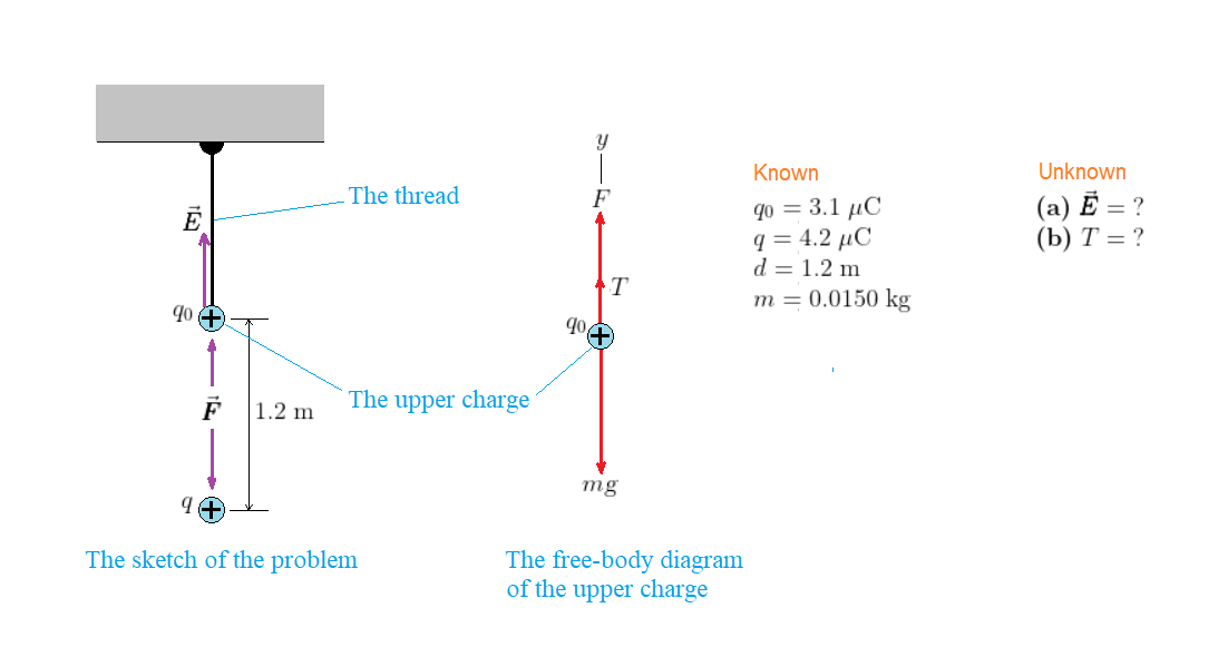
The situation is shown in our sketch, along with the free-body diagram for the thread. Notice that we choose the upward direction as the positive $y$ direction.
$text{color{#4257b2}Strategy}$
$textbf{(a)}$ The charges on the two given objects have the same sign (positive), so the electric field at the position of the upper charge (of magnitude $q_0$) due to the lower charge (of magnitude $q$) is directed upward. Moreover, it has a magnitude equal to $kq/d^2$, with $d = 1.2$ m. $textbf{(b)}$ There are three forces acting on the upper charge; its downward weight $mtextit{g}$, the upward tension $T$ in the thread, and the upward electric force $F$ exerted by the lower charge $q$. Notice that the magnitude of the electric force $F$ is equal to $q_0E$, where $E$ is the magnitude of the electric field at the position of $q_0$ due to $q$ (given by part (a)). We apply Newton’s first law to the upper charge along the vertical direction ($y$ direction) to obtain an expression for $T$ in terms of $F$ and $mtextit{g}$, from which we can find the value of $T$.
$text{color{#4257b2}Solution}$
$textbf{(a)}$ The electric field at $q_0$ due to $q$ is
$$
begin{align*}
E &= kfrac{q}{d^2}\
&= (8.99times10^9;mathrm{N}cdotmathrm{m}^2/mathrm{C}^2)timesfrac{4.2times10^{-6};mathrm{C}}{(1.2;mathrm{m})^2}\
&= 2.6times10^4;mathrm{N/C}qquad text{(upward)}
end{align*}
$$
$textbf{(b)}$ We apply Newton’s first law to the upper charge in the $y$ direction:
$$
Sigma F_y = F + T – mtextit{g} = 0
$$
We solve the equation for $T$ and express $F$ as $q_0E$:
$$
begin{align*}
T &= mtextit{g} – F\
T &= mtextit{g} – q_0E
end{align*}
$$
We substitute $m = 0.0150$ kg, $q_0 = 3.1;mu$C = $3.1times10^{-6}$ C, and $E = 2.6times10^4$ N/C (from part (a)), and find $T$:
$$
begin{align*}
T &= (0.0150;mathrm{kg})(9.8;mathrm{m/s}^2) – (3.1times10^{-6};mathrm{C})(2.6times10^4;mathrm{N/C})\
&= 0.066 ;mathrm{N}
end{align*}
$$
$textbf{(a)}$ The electric potential at any of the given points is equal to the electric potential due to the positive charge in positive sign plus the electric potential due the negative charge in negative sign. As a result, the electric potential is smallest in value at the closest point to the point halfway between the two charges. $textbf{(b)}$ The given two charges have the same magnitude, but the positive charge is closer to the given points (ruling out the point A) in each case than the negative charge is. This means the total electric potential at each of the given points is positive (the electric potential is zero at A). Since the magnitude of the electric potential at any point depends inversely on the distance, it follows that the electric potential has the greatest (positive) value at that point as close as possible to the positive charge and at the same time as further as possible from the negative charge. $textbf{(c)}$ At each point of interest, the electric potential is the algebraic sum of the electric potentials due to the two charges. In particular, the electric potential due to either charge $q$ at a point $r$ distance from such charge is equal to $kq/r$.
$text{color{#4257b2}Solution}$
$textbf{(a)}$ The point A (located at the origin) is exactly halfway between the two opposite-in-sign charges. Hence, the electric potential is smallest in value (numerically zero) at A.
$textbf{(b)}$ The remaining points, B, C, and D, are all the same distance from the positive charge. However, from the geometry of Fig. 20.34 the points B and D are the same distance from the negative charge, which is $smaller$ in length than that of point C from the negative charge (this comes as a consequence of the triangle inequality). Hence, the electric potential due to the negative charge at C is the least negative, which when combined with the positive potential gives an ultimate electric potential at C as the most positive (having the greatest value).
At point C, the electric potential due to the positive charge is $V_+ = +k|q|/r_+$, with $|q| = 1.2;mu$C and $r_+ = 0.50$ m and the electric potential due to the negative charge is $V_- = -k|q|/r_-$, with $|q| = 1.2;mu$C and $r_- = 1.5$ m. In such case, the electric potential at C is the sum $V_{rm C} = V_+ + V_-$:
$$
begin{align*}
V_{rm C} &= +kfrac{|q|}{r_+} – kfrac{|q|}{r_-}\
&= k|q|left(frac{1}{r_+} – frac{1}{r_-}right)\
&= (8.99times10^9;mathrm{N}cdotmathrm{m}^2/mathrm{C}^2)(1.2times10^{-6};mathrm{C})\
×left(frac{1}{0.50;mathrm{m}} – frac{1}{1.5;mathrm{m}}right)\
&= 14;mathrm{kV}
end{align*}
$$
The points B and D are the same distance from each of the two charges. Hence, the total electric potential at either point is the same and equal to the positive electric potential $V_+ = +k|q|/r_+$, with $|q| = 1.2;mu$C and $r_+ = 0.50$ m, plus the negative electric potential $V_- = -k|q|/r_-$, with $|q| = 1.2;mu$C and $r_- = sqrt{(1.0;mathrm{m})^2 + (0.50;mathrm{m})^2} = 1.1$ m. That the electric potential at B or D is
$$
begin{align*}
V_{rm B} = V_{rm D} &= +kfrac{|q|}{r_+} – kfrac{|q|}{r_-}\
&= k|q|left(frac{1}{r_+} – frac{1}{r_-}right)\
&= (8.99times10^9;mathrm{N}cdotmathrm{m}^2/mathrm{C}^2)(1.2times10^{-6};mathrm{C})\
×left(frac{1}{0.50;mathrm{m}} – frac{1}{1.1;mathrm{m}}right)\
&= 12;mathrm{kV}
end{align*}
$$
$text{color{#4257b2}Insight}$
As we see from the results of part (c), the electric potential does have its smallest value at point A and its greatest value at point C.
$textbf{(b)}$ C
$textbf{(c)}$ 0, 12 kV, 14 kV, 12 kV
$textbf{(a)}$ The electric potential at any of the given points are the sum of the positive-signed values of the electric potentials due to the individual positive charges. As a result, the electric potential is smallest in value at the point located as further as possible from the location of each charge. $textbf{(b)}$ In contrast to part (a), the electric potential has its greatest value at the point the closest possible to the location of each charge. $textbf{(c)}$ At each point of interest, the electric potential is the sum of the electric potentials due to each individual charge. In particular, the electric potential due to either charge $q$ at a point distance $r$ from the location of $q$ is equal to $kq/r$.
$text{color{#4257b2}Solution}$
$textbf{(a)}$ Referring to the geometry of Fig. 20.34, the point C is the farthest possible from the location of each charge (again the triangle inequality comes into the scene). Hence, the electric potential is smallest in value at C.
$textbf{(b)}$ The point A is the closest possible to the location of each charge. Hence, the electric potential must have its greatest value at A.
$$
begin{align*}
V_{rm A} &= 2kfrac{q}{r}\
&= 2(8.99times10^9;mathrm{N}cdotmathrm{m}^2/mathrm{C}^2)timesfrac{1.2times10^{-6};mathrm{C}}{0.50;mathrm{m}}\
&= 43;mathrm{kV}
end{align*}
$$
At point C, the electric potential is the sum of the electric potential due to the left charge, $V_{ell} = +kq/r_{ell}$, with $q = 1.2;mu$C and $r_ell = 1.5$ m, and the electric potential due to the right charge, $V_{rm r} = +kq/r_{rm r}$, with $q = 1.2;mu$C and $r_{rm r} = 0.50$ m:
$$
begin{align*}
V_{rm C} &= kfrac{q}{r_ell} + kfrac{q}{r_{rm r}}\
&= kqleft(frac{1}{r_ell} + frac{1}{r_{rm r}}right)\
&= (8.99times10^9;mathrm{N}cdotmathrm{m}^2/mathrm{C}^2)(1.2times10^{-6};mathrm{C})times\
&left(frac{1}{1.5;mathrm{m}} + frac{1}{0.50;mathrm{m}}right)\
&= 29;mathrm{kV}
end{align*}
$$
The points B and D are the same distance from the location of each charge. Hence, the total electric potential at either point has the same value, which is equal to the electric potential due to the left charge, $V_{ell} = +kq/r_{ell}$, with $q = 1.2;mu$C and $r_ell = sqrt{(1.0;mathrm{m})^2 + (0.50;mathrm{m})^2} = 1.1$ m, plus the electric potential due to the right charge, $V_{rm r} = +kq/r_{rm r}$, with $q = 1.2;mu$C and $r_{rm r} = 0.50$ m:
$$
begin{align*}
V_{rm B} = V_{rm D} &= kfrac{q}{r_ell} + kfrac{q}{r_{rm r}}\
&= kqleft(frac{1}{r_ell} + frac{1}{r_{rm r}}right)\
&= (8.99times10^9;mathrm{N}cdotmathrm{m}^2/mathrm{C}^2)(1.2times10^{-6};mathrm{C})times\
&left(frac{1}{1.1;mathrm{m}} + frac{1}{0.5;mathrm{m}}right)\
&= 31;mathrm{kV}
end{align*}
$$
As we see from the results of part (c), the electric potential does have its smallest value at point C and its greatest value at point A.
$textbf{(b)}$ A
$textbf{(c)}$ 43 kV, 31 kV, 29 kV, 31 kV
$$
begin{aligned}
Sigma F_{text{net}}=ma
end{aligned}
$$
such that $Sigma F_text{net}$ is the summation of the forces acting on the a body.
$$
begin{aligned}
Sigma F_{text{net}}=F_text{g}-F_text{e}=mg-qE
end{aligned}
$$
wherein $F_text{g}$ is the force of gravity acting on the ball and $F_text{e}$ is the opposing electric force.
$$
begin{aligned}
E=-frac{Delta V}{d}
end{aligned}
$$
$$
begin{aligned}
Sigma F_{text{net}}&=mg+qfrac{Delta V}{d}=ma \
Delta V&=frac{m(a-g)d}{q} tag{1}
end{aligned}
$$
$$
begin{aligned}
y=y_0+v_0t-frac{1}{2}gt^2
end{aligned}
$$
$$
begin{aligned}
g&=-frac{2(y-y_0-v_0t)}{t^2} \& =-frac{2(0;text{m}-1.00text{m}-(0;text{m/s})(0.552;text{s}))}{(0.552;text{s})^2} \ &=6.56;text{m}/text{s}^2
end{aligned}
$$
$$
begin{aligned}
a&=-frac{2(y-y_0-v_0t)}{t^2} \ &=-frac{2(0;text{m}-1.00text{m}-(0;text{m/s})(0.680;text{s}))}{(0.680;text{s})^2} \ &=4.33;text{m}/text{s}^2
end{aligned}
$$
$$
begin{aligned}
Delta V&=frac{m(a-g)d}{q}\&=frac{(0.250;text{kg})(4.33;text{m}/text{s}^2-6.56;text{m}/text{s}^2)(1.00;text{m})}{7.75times10^{-6};text{C}}\&=-7.22times10^{4};text{V}
end{aligned}
$$
$$
begin{aligned}
Delta V&=V_text{f}-V_text{i}\
V_text{i}&=V_text{f}-Delta V\&=0;text{V}-(-7.22times10^{4};text{V})\&=boxed{7.22times10^{4};text{V}}
end{aligned}
$$
$$
begin{aligned}
x_text{f}&=x_text{i}+v_text{x,i}t\
y_text{f}&=y_text{i}+v_text{y,i}t-frac{1}{2}a_text{y}t^2
end{aligned}
$$
$$
begin{aligned}
t=frac{x_text{f}-x_text{i}}{v_text{x,i}}=frac{2.25times10^{-2};text{m}-0;text{m}}{5.45times10^6;text{m/s}}=4.1times10^{-9};text{s}
end{aligned}
$$
$$
begin{aligned}
y_text{f}&=y_text{i}-frac{1}{2}a_text{y}t^2\
a_text{y}&=2frac{y_text{i}-y_text{f}}{t^2}
end{aligned}
$$
$$
begin{aligned}
Sigma F_text{y}=ma_text{y}\
F_text{e}=ma_text{y}\
a_text{y}=frac{F_text{e}}{m}
end{aligned}
$$
$$
begin{aligned}
a_text{y}=frac{Eq_0}{m}
end{aligned}
$$
$$
begin{aligned}
frac{Eq_0}{m}&=2frac{y_text{i}-y_text{f}}{t^2}\
E&=2frac{m(y_text{i}-y_text{f})}{q_0t^2}
end{aligned}
$$
$$
begin{aligned}
E&=2left(frac{9.11times10^{-31};text{kg}(0;text{m}-(-0.618times10^{-2};text{m}))}{(1.60times10^{-19};text{C})(4.1times10^{-9};text{s})^2}right)\&=boxed{4129;text{N/C}}
end{aligned}
$$
$$
begin{aligned}
V=kfrac{q}{r}
end{aligned}
$$
where $k=8.99times10^{9}text{N}cdottext{m}^2/text{C}^2$. To obtain $r$, we can use the distance formula:
$$
begin{aligned}
r=sqrt{(x_2-x_1)^2+(y_2-y_1)^2}
end{aligned}
$$
$$
begin{aligned}
r_1=sqrt{(4.40;text{m}-0;text{m})^2+(6.22;text{m}-0;text{m})^2}=7.62;text{m}
end{aligned}
$$
$$
begin{aligned}
r_2=sqrt{(-4.50;text{m}-0;text{m})^2+(6.75;text{m}-0;text{m})^2}=8.11;text{m}
end{aligned}
$$
$$
begin{aligned}
r_3=sqrt{(2.23;text{m}-0;text{m})^2+(-3.31;text{m}-0;text{m})^2}=3.99;text{m}
end{aligned}
$$
$$
begin{aligned}
V=V_1 + V_2 + V_3 = kfrac{q_1}{r_1}+kfrac{q_2}{r_2}+kfrac{q_3}{r_3}
end{aligned}
$$
$$
begin{aligned}
0&=kfrac{q_1}{r_1}+kfrac{q_2}{r_2}+kfrac{q_3}{r_3}\
0&=frac{q_1}{r_1}+frac{q_2}{r_2}+frac{q_3}{r_3}\
frac{q_3}{r_3}&=-left(frac{q_1}{r_1}+frac{q_2}{r_2} right)\
q_3&=-r_3left(frac{q_1}{r_1}+frac{q_2}{r_2} right)
end{aligned}
$$
$$
begin{aligned}
q_3&=-(3.99;text{m})left(frac{24.5times 10 ^{-6}text{C}}{7.62;text{m}}+frac{-11.2times 10 ^{-6}text{C}}{8.11;text{m}} right)\&=boxed{-7.32;mutext{C}}
end{aligned}
$$
$$
begin{aligned}
Q=CV
end{aligned}
$$
where $C$ is the capacitance of the capacitor and $V$ is the electric potential difference.
$$
begin{aligned}
Q&=(7.6times10^{-12};text{F})(650;text{V})\&=boxed{4.9times10^{-9};text{C}}
end{aligned}
$$
$$
begin{aligned}
PE=frac{1}{2}QV
end{aligned}
$$
$$
begin{aligned}
PE&=frac{1}{2}(4.9times10^{-9};text{C})(650;text{V})\
&=boxed{1.6times10^{-6};text{J}}
end{aligned}
$$
