First investment:

$A=2500(1+0.082)^{24}=$16572.74$

Second investment:

$A=2500(1+0.082)^{23}=$14,155.97$

Third investment:

$A=2500(1+0.082)^{22}=$13,083.15$

Fourth investment:

$$
A=2500(1+0.082)^{21}=$13083.15
$$

$A=P(1+i)^{m}$

where

$A$ = future value

$P$ = principal or initial value

$i$ = interest rate per compounding period

$m$ = number of compounding periods

$$
r=1.082
$$

$t_1+t_2+t_3+t_4+…+t_{n-1}+t_n$ is

$$
t_n=a_1cdot r^{n-1}
$$

$FV=2500$

$i=0.082$

$m=25$

The future value of the annuity is

$$
FV=2500cdot dfrac{1.082^{25}-1}{0.082}=$188,191.50
$$

$FV=Rcdot dfrac{(1+i)^m-1}{i}$

where

$FV$ = future value of the annuity

$R$ = recurring payment

$i$ = interest rate per compounding

$m$ = number of compounding periods

b.) $r=1.082$

c.) $$188,191.50$

$FV=Rcdot dfrac{(1+i)^m-1}{i}$

where

$FV$ = future value of the annuity

$R$ = recurring payment

$i$ = interest rate per compounding

$m$ = number of compounding periods

$FV = 100cdot dfrac{1.003^{600}-1}{0.003}=$167;778.93$

$FV=1500cdot dfrac{1.0155^{60}-1}{0.0155}=$146;757.35$

$FV=500cdot dfrac{1.028^{16}-1}{0.028}=$9920.91$

$$
FV=4000cdot dfrac{1.045^{10}-1}{0.045}=$49;152.84
$$

b.) $$146;757.35$

c.) $$9;920.91$

d.) $$49;152.84$

$FV=Rcdot dfrac{(1+i)^m-1}{i}$

where

$FV$ = future value of the annuity

$R$ = recurring payment

$i$ = interest rate per compounding

$m$ = number of compounding periods

$R=650$

$i=0.023$

The future value is

$FV=650cdot dfrac{1.023^{50}-1}{0.023}=$59,837.37$

To obtain the interest, we shall find subtract the future value with the total amount invested.

$P=650times 50=$32;500$

$I=FV-P=59837.37-32500=boxed{bold{$27;837.37}}$

Lois earned an interest of $$27,837.37$

$FV=Rcdot dfrac{(1+i)^m-1}{i}$

where

$FV$ = future value of the annuity

$R$ = recurring payment

$i$ = interest rate per compounding

$m$ = number of compounding periods

Normally, the annual interest rate $r$, number of years $t$, and the compounding mode is given, in that case, use the following formula

$i=dfrac{r}{n}$

$m=ncdot t$

$$
n = left{ {begin{array}{c}
{1;;{text{for annually}}} \
{2{text{ for semi-annually}}} \
{4{text{ for quarterly}}} \
{12{text{ for monthly}}}
end{array}} right.
$$

$R=650$

$r=0.054$ compounded monthly for 3 years

Solve for $i$ and $m$

$i=dfrac{r}{n}=dfrac{0.054}{12}=0.0045$

$m=12cdot 3=36$

We can now calculate the future value of annuity

$FV=Rcdot dfrac{(1+i)^m-1}{i}$

$$
FV=125.45times dfrac{1.0045^{36}-1}{0.0045}=bold{bf{$4,889.90}}
$$

$FV=Rcdot dfrac{(1+i)^m-1}{i}$

where

$FV$ = future value of the annuity

$R$ = recurring payment

$i$ = interest rate per compounding

$m$ = number of compounding periods

If the annual interest rate $r$, number of years $t$, and the compounding mode is given, in that case, use the following formula

$i=dfrac{r}{n}$

$m=ncdot t$

$$
n = left{ {begin{array}{c}
{1;;{text{for annually}}} \
{2{text{ for semi-annually}}} \
{4{text{ for quarterly}}} \
{12{text{ for monthly}}}
end{array}} right.
$$

$R=1500$, $i=0.063$ , $m=10$

$FV=Rcdot dfrac{(1+i)^m-1}{i}$

$$
FV=1500cdot dfrac{1.063^{10}-1}{0.063}=$20;051.96
$$

$R=250$ , $i=0.018$ , $m=6$

$FV=Rcdot dfrac{(1+i)^m-1}{i}$

$$
FV=250cdot dfrac{1.018^6-1}{0.018}=$1;569.14
$$

$R=2400$ , $i=0.012$ , $m=28$

$FV=Rcdot dfrac{(1+i)^m-1}{i}$

$$
FV=2400cdot dfrac{1.012^{28}-1}{0.012}=$79;308.62
$$

$R=25$ , $i=dfrac{2}{300}$ , $m=420$

$FV=Rcdot dfrac{(1+i)^m-1}{i}$

$$
FV=25cdot dfrac{left(1+dfrac{2}{300}right)-1}{left(dfrac{2}{300}right)}=$57;347.07
$$

b.) $$1;569.14$

c.) $$79;308.62$

d.) $$57;347.07$

$FV=Rcdot dfrac{(1+i)^m-1}{i}$

where

$FV$ = future value of the annuity

$R$ = recurring payment

$i$ = interest rate per compounding

$m$ = number of compounding periods

If the annual interest rate $r$, number of years $t$, and the compounding mode is given, in that case, use the following formula

$i=dfrac{r}{n}$

$m=ncdot t$

$$
n = left{ {begin{array}{c}
{1;;{text{for annually}}} \
{2{text{ for semi-annually}}} \
{4{text{ for quarterly}}} \
{12{text{ for monthly}}}
end{array}} right.
$$

$FV=Rcdot dfrac{(1+i)^m-1}{i}implies R=dfrac{FVcdot i }{(1+i)^m-1}$

$$
R=dfrac{1,000,000cdot (0.0085)}{(1+0.0085)^{480}-1}=$148.77
$$

$FV=Rcdot dfrac{(1+i)^m-1}{i}implies R=dfrac{FVcdot i }{(1+i)^m-1}$

$$
R=dfrac{1,000,000cdot (0.000425)}{(1+0.000425)^{480}-1}=$638.38
$$

b.) $$638.38$

$FV=Rcdot dfrac{(1+i)^m-1}{i}$

where

$FV$ = future value of the annuity

$R$ = recurring payment

$i$ = interest rate per compounding

$m$ = number of compounding periods

If the annual interest rate $r$, number of years $t$, and the compounding mode is given, in that case, use the following formula

$i=dfrac{r}{n}$

$m=ncdot t$

$$
n = left{ {begin{array}{c}
{1;;{text{for annually}}} \
{2{text{ for semi-annually}}} \
{4{text{ for quarterly}}} \
{12{text{ for monthly}}}
end{array}} right.
$$

$FV=Rcdot dfrac{(1+i)^m-1}{i}$

where

$FV$ = future value of the annuity

$R$ = recurring payment

$i$ = interest rate per compounding

$m$ = number of compounding periods

If the annual interest rate $r$, number of years $t$, and the compounding mode is given, in that case, use the following formula

$i=dfrac{r}{n}$

$m=ncdot t$

$$
n = left{ {begin{array}{c}
{1;;{text{for annually}}} \
{2{text{ for semi-annually}}} \
{4{text{ for quarterly}}} \
{12{text{ for monthly}}}
end{array}} right.
$$

$r=5.2%=0.052$

$R=250$

We need to find the number of years $t$ needed to achieve $FV=6500$ for quarterly compounding (n=4)

$i=dfrac{r}{n}=dfrac{0.052}{4}=0.013$

$m=ntimes t=4t$

Using the formula

$FV=Rcdot dfrac{(1+i)^m-1}{i}$

$dfrac{FVcdot i}{R}=(1+i)^m-1$

$(1+i)^m=dfrac{FVcdot i}{R}+1$

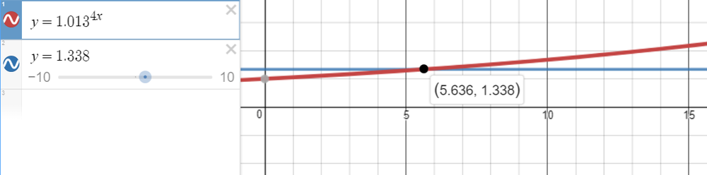
$(1.013)^{4t}=dfrac{6500(0.013)}{250}+1$

$(1.013)^{4t}=1.338$

We shall solve it graphically.

$FV=Rcdot dfrac{(1+i)^m-1}{i}$

where

$FV$ = future value of the annuity

$R$ = regular recurring payment

$i$ = interest rate per compounding

$m$ = number of compounding periods

If the annual interest rate $r$, number of years $t$, and the compounding mode is given, in that case, use the following formula

$i=dfrac{r}{n}$

$m=ncdot t$

$$
n = left{ {begin{array}{c}
{1;;{text{for annually}}} \
{2{text{ for semi-annually}}} \
{4{text{ for quarterly}}} \
{12{text{ for monthly}}}
end{array}} right.
$$

$FV=Rcdot dfrac{(1+i)^m-1}{i}$

$R=dfrac{FV cdot i}{(1+i)^m-1}$

Sonia: $R=dfrac{500,000cdot 0.0055}{(1+0.0055)^{420}-1}=$305.19$

Anita: $R=dfrac{500,000cdot 0.009}{(1+0.009)^{420}-1}=$106.94$

The difference is

$305.19-106.94=boxed{bf{$198.25}}$

Therefore, to achieve the same result, Sonja should invest $$198.25$ per month more than Anita.

$FV=305.19cdot dfrac{(1.009)^{420}-1}{0.009}=1,426,980.31$

The difference is

$1,426,980.31-500,000=boxed{bf{$926,980.31}}$

Thus Anita will earn $$926,980.31$ more than Sonja.

b.) Anita will earn $$926,980.31$ more than Sonja

$FV=Rcdot dfrac{(1+i)^m-1}{i}$

where

$FV$ = future value of the annuity

$R$ = regular recurring payment

$i$ = interest rate per compounding

$m$ = number of compounding periods

If the annual interest rate $r$, number of years $t$, and the compounding mode is given, in that case, use the following formula

$i=dfrac{r}{n}$

$m=ncdot t$

$$
n = left{ {begin{array}{c}
{1;;{text{for annually}}} \
{2{text{ for semi-annually}}} \
{4{text{ for quarterly}}} \
{12{text{ for monthly}}}
end{array}} right.
$$

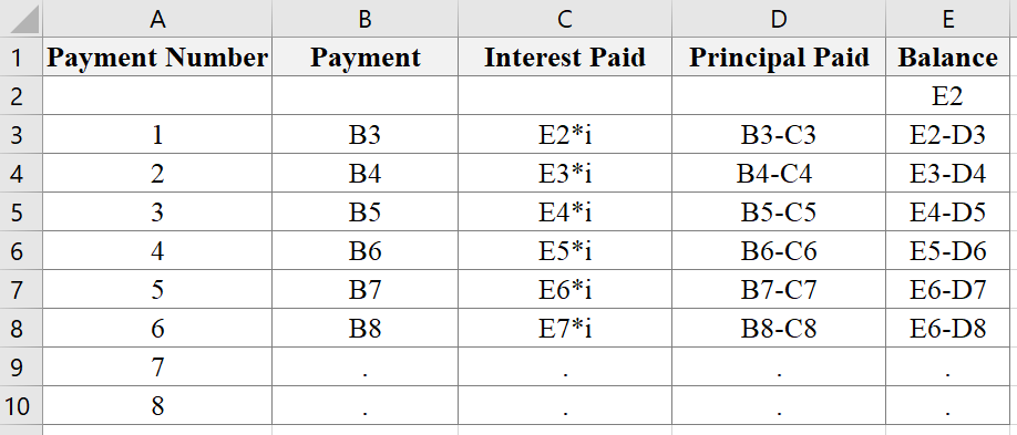
(1) Payment Number

(2) Payment (if not given, solve for R using the formula above)

(3) Interest Paid = Previous Balance $times$ Interest Rate per Payment Period

(4) Principal Paid = Recurring Payment $-$ Interest Paid

(5) Balance = Previous Balance $-$ Principal Paid

A sample spreadsheet is illustrated below.

$P=10,000$

$R=250$

monthly payments

$r=4.8%implies i=0.048/12=0.004$

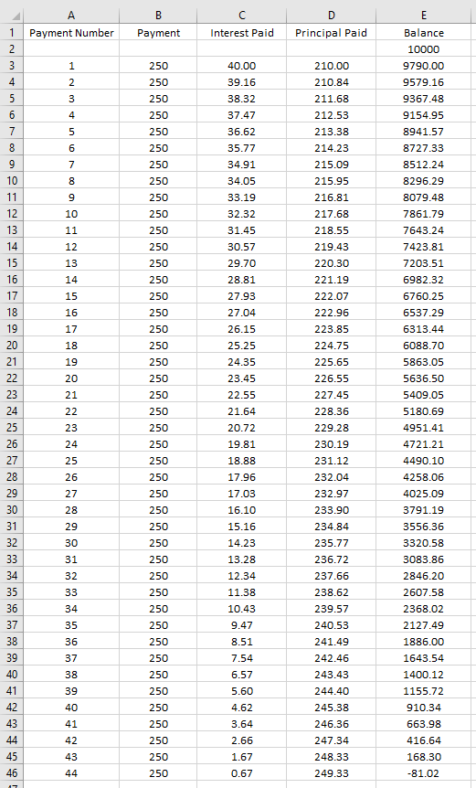
Thus, Carmen paid a total of $43times 250+168.98=$10,918.97$

The total interest is

$$
10,918.98-10,000=$918.98
$$

b.) $$918.98$

$FV=Rcdot dfrac{(1+i)^m-1}{i}$

where

$FV$ = future value of the annuity

$R$ = regular recurring payment

$i$ = interest rate per compounding

$m$ = number of compounding periods

If the annual interest rate $r$, number of years $t$, and the compounding mode is given, in that case, use the following formula

$i=dfrac{r}{n}$

$m=ncdot t$

$$
n = left{ {begin{array}{c}
{1;;{text{for annually}}} \
{2{text{ for semi-annually}}} \
{4{text{ for quarterly}}} \
{12{text{ for monthly}}}
end{array}} right.
$$

We need to find how much $R$ is need to pay for

$P=123000$

$t=20$ years

$r=6.6%implies i=0.066/12=0.0055$

$n=12$ (monthly payment)

$m=12times 20=240$

The future value of the principal after 20 years should be equivalent to the future value of the annuity paid within 20 years.

$FV=P(1+i)^m=Rcdot dfrac{(1+i)^m-1}{i}$

$R=dfrac{P(1+i)^m}{left[dfrac{(1+i)^m-1}{i}right]}$

$R=dfrac{123000(1.0055^{240}) }{left[dfrac{(1.0055)^{240}-1}{0.0055}right] }approxboxed{bf{$924.32}}$

A regular payment of $924.32$ must be done per month for 20 years.

$FV=Rcdot dfrac{(1+i)^m-1}{i}$

where

$FV$ = future value of the annuity

$R$ = regular recurring payment

$i$ = interest rate per compounding

$m$ = number of compounding periods

If the annual interest rate $r$, number of years $t$, and the compounding mode is given, in that case, use the following formula

$i=dfrac{r}{n}$

$m=ncdot t$

$$
n = left{ {begin{array}{c}
{1;;{text{for annually}}} \
{2{text{ for semi-annually}}} \
{4{text{ for quarterly}}} \
{12{text{ for monthly}}}
end{array}} right.
$$

Given that the future value of the annuity is 100 times the regular payment,

$FV=100R$ and $i=0.007$

We can find the number of payments using the formula described earlier,

$FV=Rcdot dfrac{(1+i)^m-1}{i}$

$100R=Rcdot dfrac{1.007^m-1}{0.007}$

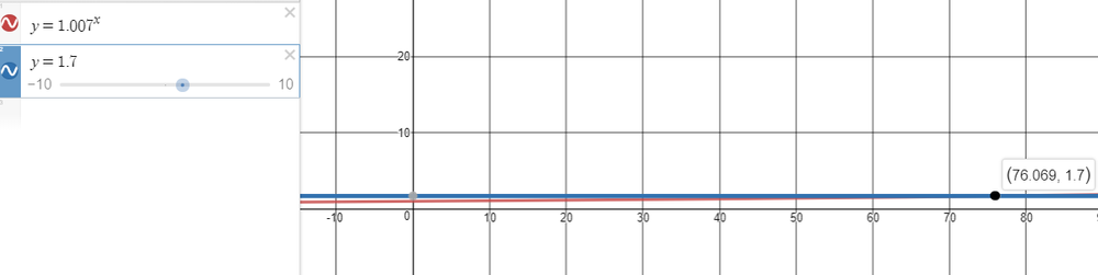
$100=dfrac{1.007^m-1}{0.007}$

$1.007^m=100(0.007)+1$

$1.007^m=1.7$