All Solutions
Page 404: Practice Questions
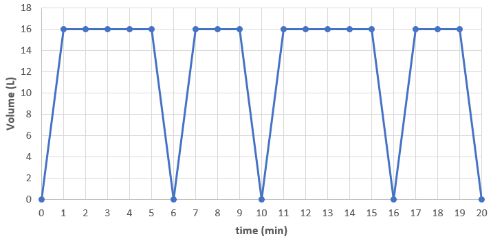
c) From the graph, each cycle takes 10 min. Thus, the period is 10 min.
It represents the time required for each cycle (in this case, batch of dishes to be washed).
d) equation of axis: $V=dfrac{V_{text{min}}+V_{text{max}}}{2}=dfrac{0+18}{2}implies V=9$
e) amplitude: $A=dfrac{V_{text{max}}-V_{text{min}}}{2}=dfrac{16-0}{2}=8$
f) The range is ${ V in bold{R};|;V_{text{min}}leq Vleq V_{text{max}}} implies { V in bold{R};|;0leq Vleq16}$
b) periodic
c) period: 10 min
d) equation of axis: $V=9$
e) amplitude: $A=8$
f) ${ V in bold{R};|;0leq Vleq16}$
{text{For a sinusoidal function, remember the following }} hfill \
hfill \
y = Acos left[ {kleft( {x – d} right)} right] + c{text{ }} hfill \
{text{or }} hfill \
y = Asin left[ {kleft( {x – d} right)} right] + c{text{ }} hfill \
hfill \
{text{amplitude = }}|A| = dfrac{|y_{text{max}}-y_{text{min}}|}{2}hfill \
{text{period = }}T=frac{{{{360}^ circ }}}{|k|} hfill \
{text{equation of axis:}}{text{ }},,,y = c = dfrac{y_{text{max}}+y_{text{min}}}{2} hfill \
hfill \
{text{Generally, if the maximum point is translated $d$ units to the right of the}}hfill \\
{text{$y$-axis, the equation is $y=Acos[k(x-d)^circ]+c$}}hfill \\
{text{If the minimum point is translated $d$ units to the right of the}}hfill \\
{text{$y$-axis, the equation is $y=-Acos[k(x-d)^circ]+c$}}hfill \\
{text{Note that multiple possible sinusoidal functions can describe a graph or data}}hfill \
end{gathered} ]
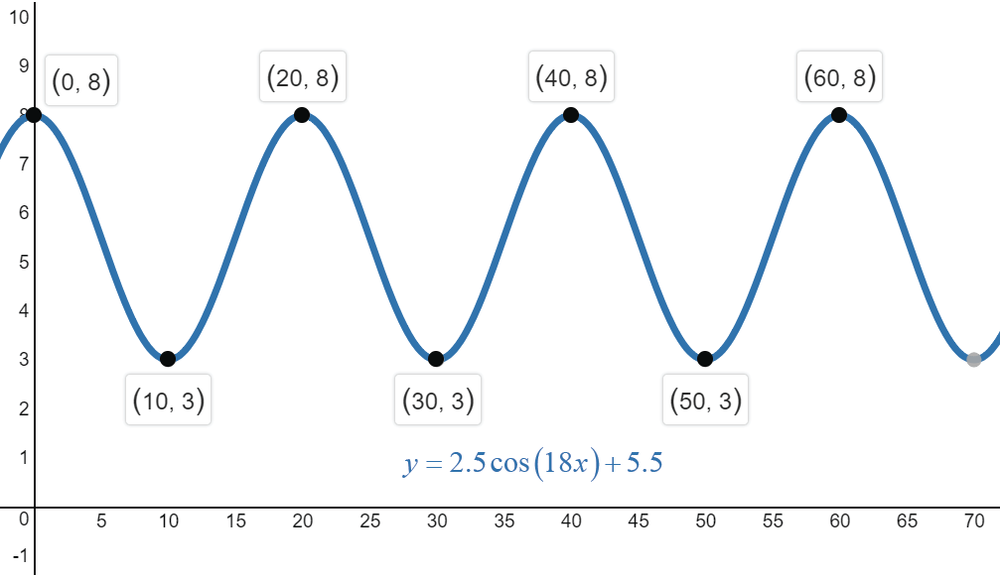
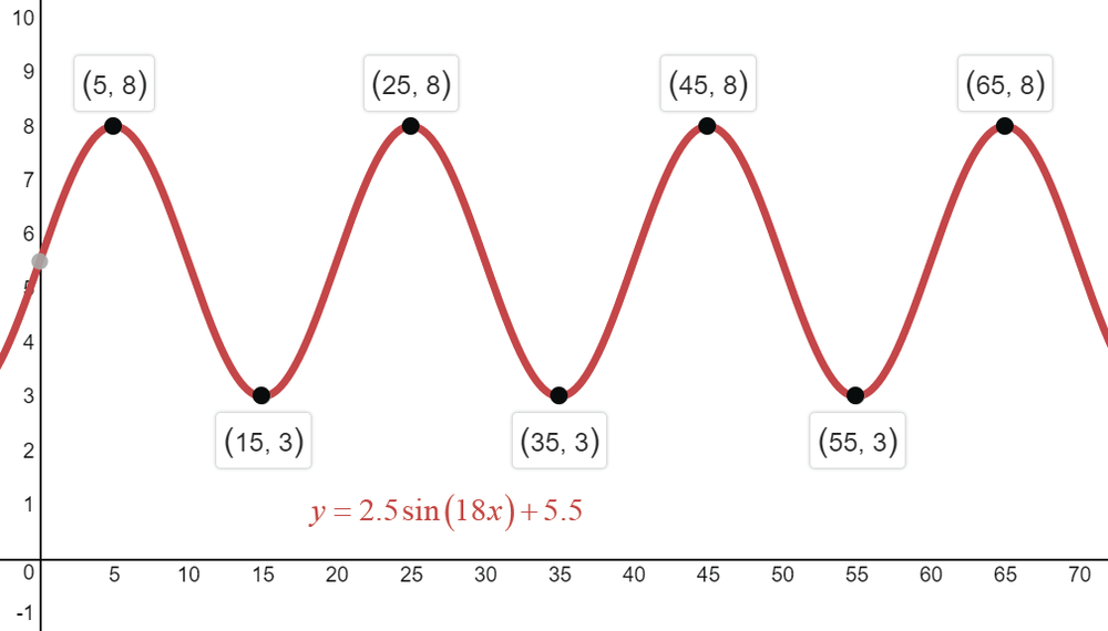
amplitude: $dfrac{|8-3|}{2}=2.5$
axis: $c=dfrac{8+3}{2}=5.5$
$k=dfrac{360^circ}{20}=18$
No restriction on the starting point is given so we can choose any horizontal translations and function (sine or cosine).
Possible answers are the graph of any of the following:
{text{For a sinusoidal function, remember the following }} hfill \
hfill \
y = Acos left[ {kleft( {x – d} right)} right] + c{text{ }} hfill \
{text{or }} hfill \
y = Asin left[ {kleft( {x – d} right)} right] + c{text{ }} hfill \
hfill \
{text{amplitude = }}|A| = dfrac{|y_{text{max}}-y_{text{min}}|}{2}hfill \
{text{period = }}T=frac{{{{360}^ circ }}}{|k|} hfill \
{text{equation of axis:}}{text{ }},,,y = c = dfrac{y_{text{max}}+y_{text{min}}}{2} hfill \
hfill \
{text{Generally, if the maximum point is translated $d$ units to the right of the}}hfill \\
{text{$y$-axis, the equation is $y=Acos[k(x-d)^circ]+c$}}hfill \\
{text{If the minimum point is translated $d$ units to the right of the}}hfill \\
{text{$y$-axis, the equation is $y=-Acos[k(x-d)^circ]+c$}}hfill \\
{text{Note that multiple possible sinusoidal functions can describe a graph or data}}hfill \
end{gathered} ]
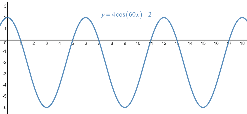
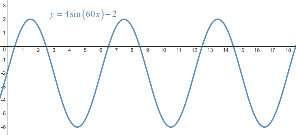
$k=dfrac{360}{6}=60$
amplitude: $A=4$
axis: $c=-2$
No restriction on the starting point are stated so we can choose any horizontal translations (that is, any value of $d$). Possible answers are:
{text{For a sinusoidal function, remember the following }} hfill \
hfill \
y = Acos left[ {kleft( {x – d} right)} right] + c{text{ }} hfill \
{text{or }} hfill \
y = Asin left[ {kleft( {x – d} right)} right] + c{text{ }} hfill \
hfill \
{text{amplitude = }}|A| = dfrac{|y_{text{max}}-y_{text{min}}|}{2}hfill \
{text{period = }}T=frac{{{{360}^ circ }}}{|k|} hfill \
{text{equation of axis:}}{text{ }},,,y = c = dfrac{y_{text{max}}+y_{text{min}}}{2} hfill \
hfill \
{text{Generally, if the maximum point is translated $d$ units to the right of the}}hfill \\
{text{$y$-axis, the equation is $y=Acos[k(x-d)^circ]+c$}}hfill \\
{text{If the minimum point is translated $d$ units to the right of the}}hfill \\
{text{$y$-axis, the equation is $y=-Acos[k(x-d)^circ]+c$}}hfill \\
{text{Note that multiple possible sinusoidal functions can describe a graph or data}}hfill \
end{gathered} ]
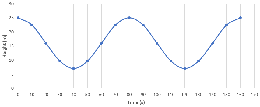
b) The equation of axis is $h=dfrac{h_{text{min}}+h_{text{max}}}{2}=dfrac{25+7}{2}implies h =16$. This represents the distance of the center of the Ferris wheel from the ground.
c) The amplitude is $A=dfrac{|25-7|}{2}=9$ which represents the radius of the Ferris wheel.
d) Yes, otherwise, the height must be constant in the first few seconds, and the graph won’t be a smooth periodic function. Furthermore, Collin is already at the top of the Ferris wheel at $t=0$ which is not possible unless it has already started moving.
e) Colin’s speed is the circumference of the Ferris wheel divided by the period: $v=dfrac{2pitimes 9;text{m}}{80;text{s}}=0.707$ m/s
f) The range is the set of values from $h_{text{min}}$ to $h_{text{max}}$
range: ${ h in bold{R};|;7leq hleq 25}$
g) The boarding height is the difference between the minimum point the height of the building which is $7-6=1$
This means Collin is at 1 m from the top of the building at the time of boarding.
b) $h=16$
c) $A=9$
d) Yes
e) $0.707$ m/s
f) ${ h in bold{R};|;7leq hleq 25}$
g) 1 m
{text{For a sinusoidal function, remember the following }} hfill \
hfill \
y = Acos left[ {kleft( {x – d} right)} right] + c{text{ }} hfill \
{text{or }} hfill \
y = Asin left[ {kleft( {x – d} right)} right] + c{text{ }} hfill \
hfill \
{text{amplitude = }}|A| = dfrac{|y_{text{max}}-y_{text{min}}|}{2}hfill \
{text{period = }}T=frac{{{{360}^ circ }}}{|k|} hfill \
{text{equation of axis:}}{text{ }},,,y = c = dfrac{y_{text{max}}+y_{text{min}}}{2} hfill \
hfill \
end{gathered} ]

equation of axis: $h(x)=9$
amplitude: $A=4$
range: ${ h(x) in bold{R};|;5leq h(x)leq 13}$
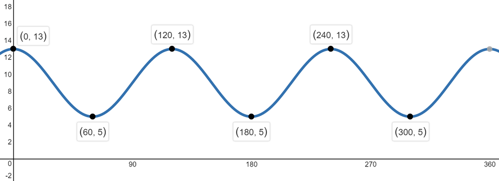
c) $h(45)=4cos[3(45)^circ]+9approx 6.17$
d) From the graph, we see that $h(x)=5$ when $x={ 60,;180,;300}$
b) Yes
c) $h(45)=6.17$
d) $x={ 60,;180,;300}$
{text{For a sinusoidal function, remember the following }} hfill \
hfill \
y = Acos left[ {kleft( {x – d} right)} right] + c{text{ }} hfill \
{text{or }} hfill \
y = Asin left[ {kleft( {x – d} right)} right] + c{text{ }} hfill \
hfill \
{text{amplitude = }}|A| = dfrac{|y_{text{max}}-y_{text{min}}|}{2}hfill \
{text{period = }}T=frac{{{{360}^ circ }}}{|k|} hfill \
{text{equation of axis:}}{text{ }},,,y = c = dfrac{y_{text{max}}+y_{text{min}}}{2} hfill \
hfill \
end{gathered} ]
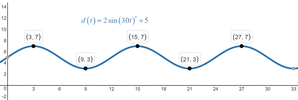
b) No waves correspond to a horizontal line at the axis $d(t)=5$.
c) $d(5.5)=2sin(30times5.5)^circ+5approx5.52$ m
d) The range is the set of possible values from $d(t)_{text{min}}$ to $d(t)_{text{max}}$
range: ${ d(t) in bold{R};|;3leq d(t) leq 7}$
e) We see from the graph that within first 10s, $d(t)=3$ only once at $t=9$ s
b) 5 m
c) 5.52 m
d) ${ d(t) in bold{R};|;3leq d(t) leq 7}$
e) $t=9$ s
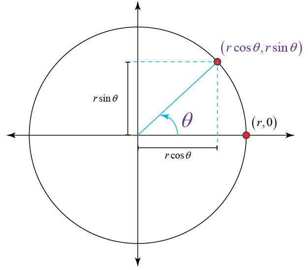
$x=4cos 25approx 3.62$
$y=4sin 25approx 1.69$
Thus, the coordinate of the new point is (3.62,1.69)
defarraystretch{1.5}%
begin{tabular}{|l|l|}
hline
Transformation & Description \ hline
$y=f(x)+c$ & begin{tabular}[c]{@{}l@{}}vertical translation of\ $c$ units upwardend{tabular} \ hline
$y=f(x+d)$ & begin{tabular}[c]{@{}l@{}}horizontal translation of $d$ units\ to the leftend{tabular} \ hline
$y=acdot f(x)$ & begin{tabular}[c]{@{}l@{}}vertical stretching, multiplies\ the amplitude by $a$end{tabular} \ hline
$y=f(kx)$ & begin{tabular}[c]{@{}l@{}}horizontal compression, divides\ the period by $k$end{tabular} \ hline
$y=-f(x)$ & begin{tabular}[c]{@{}l@{}}reflecting the function in\ the $x$-axisend{tabular} \ hline
$y=f(-x)$ & begin{tabular}[c]{@{}l@{}}reflecting the function in \ the $y$-axisend{tabular} \ hline
end{tabular}
end{table}
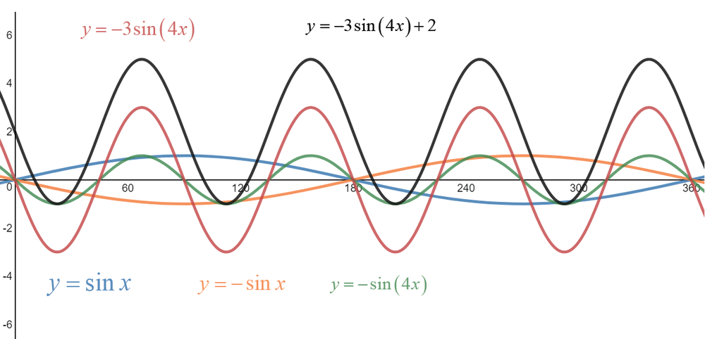
$implies$ vertical translation of 3 units downward
The equation of axis is shifted 3 units downward.
b) $y=sin(4x)$
$implies$ horizontal compression by a factor of 4.
The period is divided by 4.
c) $y=7cos x$
$implies$ vertical stretching by a factor of 7.
The amplitude is multiplied by 7.
d) $y=cos(x-70^circ)$
$implies$ Horizontal translation to the right by $70^circ$.
It has NO effect on amplitude, axis, and period.
b) period is divided by 4
c) amplitude is multiplied by 7
d) no effect on amplitude, axis, and period
defarraystretch{1.5}%
begin{tabular}{|l|l|}
hline
Transformation & Description \ hline
$y=f(x)+c$ & begin{tabular}[c]{@{}l@{}}vertical translation of\ $c$ units upwardend{tabular} \ hline
$y=f(x+d)$ & begin{tabular}[c]{@{}l@{}}horizontal translation of $d$ units\ to the leftend{tabular} \ hline
$y=acdot f(x)$ & begin{tabular}[c]{@{}l@{}}vertical stretching, multiplies\ the amplitude by $a$end{tabular} \ hline
$y=f(kx)$ & begin{tabular}[c]{@{}l@{}}horizontal compression, divides\ the period by $k$end{tabular} \ hline
$y=-f(x)$ & begin{tabular}[c]{@{}l@{}}reflecting the function in\ the $x$-axisend{tabular} \ hline
$y=f(-x)$ & begin{tabular}[c]{@{}l@{}}reflecting the function in \ the $y$-axisend{tabular} \ hline
end{tabular}
end{table}
(1) horizontally compress by a factor of 2 (divide period by 2)
(2) vertically stretch by a factor of 5 (multiply amplitude by 5)
(3) vertically translate upwards by 7
(1) reflect over $x$-axis
(2) horizontally compress by a factor of 4 (divide the period by 4)
(3) vertically stretch by a factor of 3 (multiply the amplitude by 3)
(4) vertically translate upwards by 2
$y=Acos[k(x-d)]+c$
or
$y=Asin[k(x-d)]+c$
The range is
$$
{ y in bold{R} ;|;c-|A| leq y leq c+|A|}
$$
From the equation, $A=-3$, $c=2$
$c-|A|=2-|-3|=-1$
$c-|A|=2+|3|=5$
Therefore, using the formula mentioned above
$$
{ yin bold{R};| -1 leq y leq 5}
$$
From the equation, $A=0.5$ , $c=0$
$c-|A|=0-0.5=-0.5$
$c+|A|=0+0.5=0.5$
$$
{ yin bold{R};|;-0.5leq yleq 0.5}
$$
b) ${ yin bold{R};|;-0.5leq yleq 0.5}$
{text{For a sinusoidal function, remember the following }} hfill \
hfill \
y = Acos left[ {kleft( {x – d} right)} right] + c{text{ }} hfill \
{text{or }} hfill \
y = Asin left[ {kleft( {x – d} right)} right] + c{text{ }} hfill \
hfill \
{text{amplitude = }}|A| = dfrac{|y_{text{max}}-y_{text{min}}|}{2}hfill \
{text{period = }}T=frac{{{{360}^ circ }}}{|k|} hfill \
{text{equation of axis:}}{text{ }},,,y = c = dfrac{y_{text{max}}+y_{text{min}}}{2} hfill \
hfill \
{text{Generally, if the maximum point is translated $d$ units to the right of the}}hfill \\
{text{$y$-axis, the equation is $y=Acos[k(x-d)^circ]+c$}}hfill \\
{text{If the minimum point is translated $d$ units to the right of the}}hfill \\
{text{$y$-axis, the equation is $y=-Acos[k(x-d)^circ]+c$}}hfill \\
{text{Note that multiple possible sinusoidal functions can describe a graph or data}}hfill \
end{gathered} ]
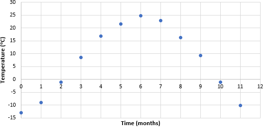
The cycle repeats every year so the behavior can be expressed by a periodic function.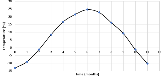
minimum is $-13.1^circ$ C which occurs in January
d) The period is 12 months (1 year). This period is appropriate because the climate cycle repeats every 1 year.
e) The equation of axis is $T=dfrac{T_{text{max}}+T_{text{min}}}{2}=dfrac{24.7+(-13.1)}{2}=5.8^circ$ C
f) Cosine function of the form $y=Acos[k(x-d)]+c$ has a maximum at the $y$-axis, since the maximum point in this case is shifted 6 units to the right, we have a phase shift of $6$ months. Cosine function of the form $y=-Acos[k(x-d)+c$ has a minimum at the $y$-axis, in this case, the phase shift is zero.
The maximum point is $6$ units to the right of the $y$-axis $implies d=6$
period is $12$ months $implies k=dfrac{360}{12}=30$
axis: as obtained in part(e), $c=5.8$
Using the form $y=Acos[k(x-d)]+c$, the equation describing the data is
$T=18.9cos[30(x-6)]+5.8$
$T(38)=18.9cos[30(38-6)]+5.8=-3.65^circ$ C
To use the table, we need to know what month corresponds to $38^{th}$ month.
January corresponds to 0th, 12th, 24th and 36th month. Therefore 38th month would be March which as a temperature of $-1.1^circ$ C
b) see graph inside
c) max: 24.7 $^circ$ C, min: $-13.1^circ$ C
d) 12 months
e) $T=5.8^circ$ C
f) 6 months
g) $T=18.9cos[30(x-6)]+5.8$
h) $-3.65^circ$ C
{text{For a sinusoidal function, remember the following }} hfill \
hfill \
y = Acos left[ {kleft( {x – d} right)} right] + c{text{ }} hfill \
{text{or }} hfill \
y = Asin left[ {kleft( {x – d} right)} right] + c{text{ }} hfill \
hfill \
{text{amplitude = }}|A| = dfrac{|y_{text{max}}-y_{text{min}}|}{2}hfill \
{text{period = }}T=frac{{{{360}^ circ }}}{|k|} hfill \
{text{equation of axis:}}{text{ }},,,y = c = dfrac{y_{text{max}}+y_{text{min}}}{2} hfill \
hfill \
{text{Generally, if the maximum point is translated $d$ units to the right of the}}hfill \\
{text{$y$-axis, the equation is $y=Acos[k(x-d)^circ]+c$}}hfill \\
{text{If the minimum point is translated $d$ units to the right of the}}hfill \\
{text{$y$-axis, the equation is $y=-Acos[k(x-d)^circ]+c$}}hfill \\
{text{Note that multiple possible sinusoidal functions can describe a graph or data}}hfill \
end{gathered} ]
i) period: the change in $x$ from minimum to maximum is $7-1=6$ which corresponds to a half-cycle. Thus, the period is $2times 6 =12 implies k=dfrac{360}{12}=30$
ii) amplitude: $A=dfrac{3.5-1.5}{2}=1$
iii) axis: $c=dfrac{3.5+1.5}{2}=2.5$
iv) phase shift: Remember that for standard sine function, the $y$-intercept is a point half-way between maximum and minimum point and the graph is increasing as it crosses the $y$-axis.
Since we must use $y=Asin k(theta-d)+c$, we can get $d$ by finding the distance of point from the $y$-axis that is half-way between between maximum and minimum point where the graph is increasing. From the graph we see that it occurs at $x=4$ which means the phase shift is $d=4$.
From these information, the equation is
$$
y=sin[30(x-4)^circ]+2.5
$$
i) period: The distance between two peaks is $T=3implies k=dfrac{360}{3}=120$
ii) amplitude: $A=dfrac{|6-2|}{2}=2$
iii) axis: $c=dfrac{6+2}{2}=4$
iv) phase shift: Remember that for standard sine function, the $y$-intercept is a point half-way between maximum and minimum point and the graph is increasing as it crosses the $y$-axis.
Since we must use $y=Asin k(theta-d)+c$, we can get $d$ by finding the distance of point from the $y$-axis that is half-way between between maximum and minimum point where the graph is increasing. From the graph we see that it occurs at $x=1$ which means the phase shift is $d=1$.
From these information, the equation is
$$
y=2sin[120(x-1)^circ]+4
$$
b) $y=2sin[120(x-1)^circ]+4$
{text{For a sinusoidal function, remember the following }} hfill \
hfill \
y = Acos left[ {kleft( {x – d} right)} right] + c{text{ }} hfill \
{text{or }} hfill \
y = Asin left[ {kleft( {x – d} right)} right] + c{text{ }} hfill \
hfill \
{text{amplitude = }}|A| = dfrac{|y_{text{max}}-y_{text{min}}|}{2}hfill \
{text{period = }}T=frac{{{{360}^ circ }}}{|k|} hfill \
{text{equation of axis:}}{text{ }},,,y = c = dfrac{y_{text{max}}+y_{text{min}}}{2} hfill \
hfill \
{text{Generally, if the maximum point is translated $d$ units to the right of the}}hfill \\
{text{$y$-axis, the equation is $y=Acos[k(x-d)^circ]+c$}}hfill \\
{text{If the minimum point is translated $d$ units to the right of the}}hfill \\
{text{$y$-axis, the equation is $y=-Acos[k(x-d)^circ]+c$}}hfill \\
{text{Note that multiple possible sinusoidal functions can describe a graph or data}}hfill \
end{gathered} ]
With $T=1.5implies k=dfrac{360}{1.5}=240$
b) When no one is rocking, the resting position is the average between the maximum and minimum point
$c=dfrac{d_{text{max}}+d_{text{min}}}{2}=dfrac{34+18}{2}=26$ cm
c) When Meagan rocks 40 times, the total time is $40T=40times 1.5=60$
domain: ${ t in bold{R};|;0leq t leq 60}$
d) The range is the set of possible values from $d_{text{min}}$ to $d_{text{max}}$
range: ${ dinbold{R};|;18leq dleq 34}$
e) The amplitude is $A=dfrac{|d_{text{max}}-d_{text{min}}|}{2} =dfrac{|34-18|}{2}=8$
This is the distance from the resting position to either maximum or minimum distance.
f) The maximum point is shifted $1.75$ from the $y$-axis $implies d=1.75$
$d=Acos[k(t-d)]+c$
$d=8cos[240(t-1.75)]+26$
g) at $t=8$ $implies y=8cos[240(8-1.75)]+26=30$ cm
b) 26 cm
c) domain: ${ t in bold{R};|;0leq t leq 60}$
d) range: ${ dinbold{R};|;18leq dleq 34}$
e) $A=8$
f) $y=8cos[240(x-1.75)]+26$
g) $d=30$ cm
{text{For a sinusoidal function, remember the following }} hfill \
hfill \
y = Acos left[ {kleft( {x – d} right)} right] + c{text{ }} hfill \
{text{or }} hfill \
y = Asin left[ {kleft( {x – d} right)} right] + c{text{ }} hfill \
hfill \
{text{amplitude = }}|A| = dfrac{|y_{text{max}}-y_{text{min}}|}{2}hfill \
{text{period = }}T=frac{{{{360}^ circ }}}{|k|} hfill \
{text{equation of axis:}}{text{ }},,,y = c = dfrac{y_{text{max}}+y_{text{min}}}{2} hfill \
hfill \
{text{Generally, if the maximum point is translated $d$ units to the right of the}}hfill \\
{text{$y$-axis, the equation is $y=Acos[k(x-d)^circ]+c$}}hfill \\
{text{If the minimum point is translated $d$ units to the right of the}}hfill \\
{text{$y$-axis, the equation is $y=-Acos[k(x-d)^circ]+c$}}hfill \\
{text{Note that multiple possible sinusoidal functions can describe a graph or data}}hfill \
end{gathered} ]
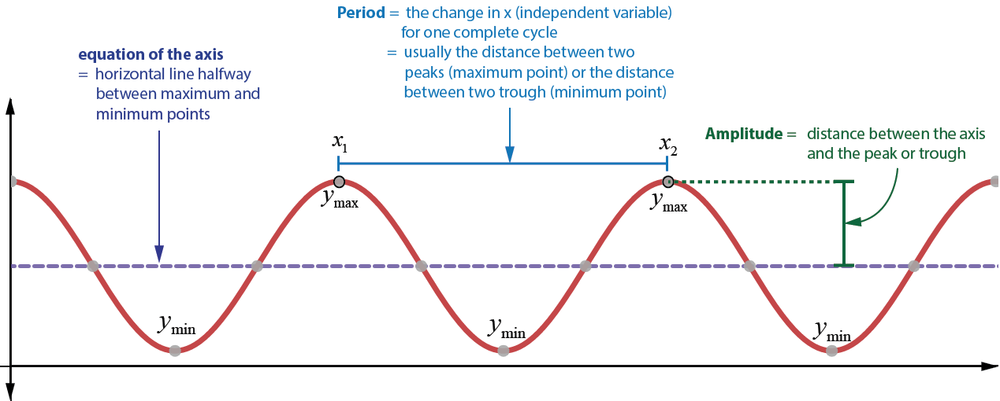
(1) period $T$: this is the change in independent variable (usually distance or time) for one complete cycle. Once the period $T$ is obtained, the value of $k$ can be calculated as $k=dfrac{360}{T}$
(2) amplitude $A$: This corresponds to the distance from the resting position to either maximum or minimum. For rotating systems (like wheels), this is usually the radius of the wheel.
(3) equation of axis: This corresponds to the resting position which is calculated as $c=dfrac{y_{text{max}}+y_{text{min}}}{2}$. In rotating systems, this is usually the distance of the center of the wheel from the ground or certain reference point.
(4) phase shift: This is the distance of the maximum point or minimum point from the $y$-axis. If the maximum point is $d$ units to the right of the $y$-intercept, the equation is $y=Acos[k(x-d)]+c$. If the minimum point is $d$ units to the right of the $y$-intercept, the equation is $y=-Acos[k(x-d)]+c$. To express the equation in terms of sine function, use the relationship $costheta=sin(90^circ-theta)$
