All Solutions
Section 1-4: Sketching Graphs of Functions
We $textbf{subtract}$ 1 from the $y$-coordinates of the parent function to $textbf{translate}$ the graph 1 unit down on $y$-axis.
#### (b)
We first $textbf{multiply}$ the $x$-coordinates of the parent function by $dfrac{1}{2}$, to apply a $textbf{horizontal compression}$ by a factor $dfrac{1}{2}$. Next,we $textbf{subtract}$ -1from the x-coordinates of the previous function,in order to $textbf{translate}$ the graph 1 unit to the right.
#### (c)
First, we $textbf{multiply}$ the $y$-coordinates by -1 to apply a $textbf{vertical strech}$ by a factor of 1. Then, $textbf{subtract}$ -3 from the $x$-coordinates and $textbf{add}$ 2 to $y$-coordinates to $textbf{translate}$ the graph 3 units to the right and 2 units up.
#### (d)
First, we $textbf{multiply}$ the $x$-coordinates of points on the parent function by $dfrac{1}{4}$, then we $textbf{multiply}$ the $y$-coordinates by -2 to apply $textbf{horizontal compression}$ by a factor of $dfrac{1}{4}$ and a $textbf{vertical strech}$ by a factor of 2.
First, we $textbf{multiply}$ the $x$-coordinates of points of the parent function by -1, then we $textbf{multiply}$ the $y$-coordinates by -1 toapply $textbf{horizontal compression}$ by -1 and $textbf{vertical strech}$ by a factor of -1. Then, $textbf{subtract}$ 2 from the $x$-coordinates and 3 from $y$-coordinates of points on the previous function, this we do to apply $textbf{transaltion}$ the graph 2 points tothe left and 3 units down.
#### (f)
First, we $textbf{multiply}$ the $x$-coordinates of points on the parent function by 4, then we $textbf{multiply}$ the $y$-coordinates by $dfrac{1}{2}$ to apply $textbf{horizontal compression}$ by 4 and $textbf{vertical strech}$ by a factor $dfrac{1}{2}$. Then,textbf{subtract} -5 from the $x$-coordinates and $textbf{add}$ 6 to the $y$-coordinates of points on the previous function. This we do to apply $textbf{translation}$ the graph 5 units to the right and 6 units up.
Representing the reflection in the $x$-axis: $a=-1$, representing the horizontal stretch by a factor of $2$: $k=dfrac{1}{2}$, representing the horizontal the horizontal translation: $d=0$, representing the vertical translation $3$ units up: $c=3$. The function is $y=-sin(dfrac{1}{2}x)+3$.
#### (b)
Representing the amplitude: $a=3$, representing the horizontal stretch by a factor of $2$: $k=dfrac{1}{2}$, representing the horizontal translation: $d=0$, representing the vertical.The function is $y=3sin(dfrac{1}{2}x)-2$.
Now, we are going to $textbf{transform coordinates}$ of point $(2,3)$ according to transformation we had at the origin function:
First, we have the transformation which follows.There is $textbf{horizontal comression}$ by $dfrac{1}{2}$,and $textbf{vertical strech}$ by a factor of -2:
$left(x,y right)rightarrowleft(dfrac{1}{2}x,-2y right)$ $Rightarrow$ $left(2,3 right)rightarrowleft(1,-6 right)$
After this, we have transformation of previous coordinates in order to make $textbf{translation}$ of the graph 5 units to the left and 4 units down:
$left(dfrac{1}{2}x,-2y right)rightarrowleft(dfrac{1}{2}x-5,-2y-4 right)$ $Rightarrow$ $left(1,-6 right)rightarrowleft(-4,-10 right)$
So, $textbf{corresponding point}$ on the graph of transformed function is $left(-4,-10 right)$
left(-4,-10 right)
$$
#### (a)
$left(x,y right)rightarrowleft(x,2y right)$, here we have $textbf{vertical strech}$ by a factor of 2.
$Rightarrow$ $left(2,3 right)rightarrowleft(2,6 right)$, $left(4,7 right)rightarrowleft(4,14 right)$, $left(-2,5 right)rightarrowleft(-2,10 right)$, $left(-4,6 right)rightarrowleft(-4,12 right)$
#### (b)
$left(x,y right)rightarrowleft(x+3,y right)$, here we have $textbf{translation}$ of the graph 3 units on the right.
$Rightarrow$ $left(2,3 right)rightarrowleft(5,3 right)$, $left(4,7 right)rightarrowleft(7,7 right)$, $left(-2,5 right)rightarrowleft(1,5 right)$, $left(-4,6 right)rightarrowleft(-1,6 right)$
#### (c)
$left(x,y right)rightarrowleft(x,y+2 right)$, here we have $textbf{translation}$ of the graph 3 units down.
$Rightarrow$ $left(2,3 right)rightarrowleft(2,5 right)$, $left(4,7 right)rightarrowleft(4,9 right)$, $left(-2,5 right)rightarrowleft(-2,7 right)$, $left(-4,6 right)rightarrowleft(-4,8 right)$
#### (d)
$left(x,y right)rightarrowleft(x-1,y-3 right)$, here we have $textbf{translation}$ of the graph 1unit on the left and 3 units down.
$Rightarrow$ $left(2,3 right)rightarrowleft(1,0 right)$, $left(4,7 right)rightarrowleft(3,4 right)$, $left(-2,5 right)rightarrowleft(-3,2right)$, $left(-4,6 right)rightarrowleft(-5,3 right)$
$left(x,y right)rightarrowleft(-x,y right)$, here we have $textbf{horizontal compression}$ by -1.
$Rightarrow$ $left(2,3 right)rightarrowleft(-2,3 right)$, $left(4,7 right)rightarrowleft(-4,7 right)$, $left(-2,5 right)rightarrowleft(2,5 right)$, $left(-4,6 right)rightarrowleft(4,6 right)$
#### (f)
$left(x,y right)rightarrowleft(dfrac{1}{2}x,y-1 right)$, here we have $textbf{horizontal compression}$ by $dfrac{1}{2}$ and $textbf{translation}$ of the graph 1 unit down.
$Rightarrow$ $left(2,3 right)rightarrowleft(1,2 right)$, $left(4,7 right)rightarrowleft(2,6 right)$, $left(-2,5 right)rightarrowleft(-1,4 right)$, $left(-4,6 right)rightarrowleft(-2,5 right)$
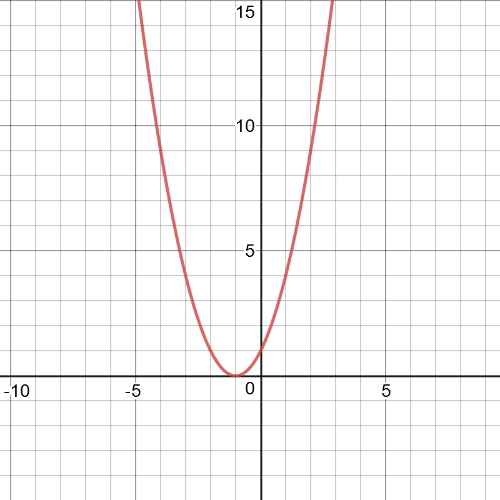
$textbf{Parent}$ function is $y=x^2$
Transformation which has been made is $textbf{translation}$ of the graph 1 unit to the left.
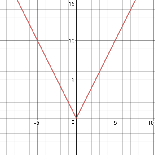
$textbf{Parent}$ function is $y=left|x right|$
Transformation which has been made is $textbf{vertical strech}$ by a factor of 2.
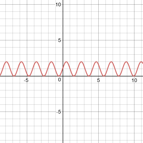
$textbf{Parent}$ function is $y=sin{x}$
Transformation which has been made is $textbf{horizontal compression}$ by $dfrac{1}{2}$ and $textbf{translation}$ the graph 1 unit up.
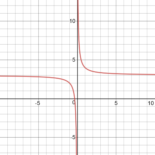
$textbf{Parent}$ function is $y=dfrac{1}{x}$
Transformation which has been made is $textbf{translation}$ the graph 3 units up.
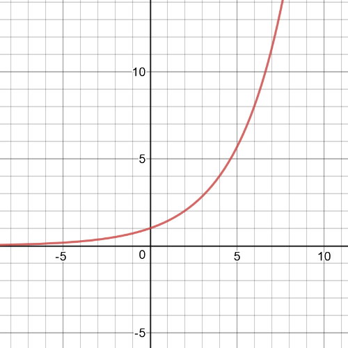
$textbf{Parent}$ function is $y=2^x$
Transformation which has been made is $textbf{horizontal compression}$ by 2.
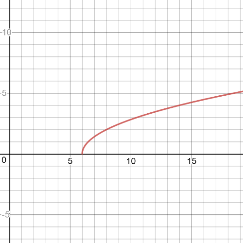
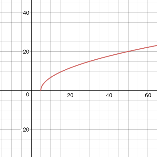
$textbf{Parent}$ function is $y=sqrt{x}$
Transformation which has been made is $textbf{horizontal compression}$ by $dfrac{1}{2}$ and $textbf{translation}$ the graph 6 units to the right.
#### (a)
$D=Bbb{R}$
$R=left[0,infty right)$
#### (b)
$D=Bbb{R}$
$R=left[0,infty right)$
#### (c)
$D=Bbb{R}$
$R=left[0,2 right]$
#### (d)
$D=Bbb{R}/left{ 0right}$
$R=Bbb{R}$
$D=Bbb{R}$
$R=left(0,infty right)$
#### (f)
$D=left[6,infty right)$
$R=left[0,infty right)$
Here we have $textbf{graphs of the parent and transformed function}$.Red one is graph of parent function $y=2^x$ and blue one is graph of transformed function.
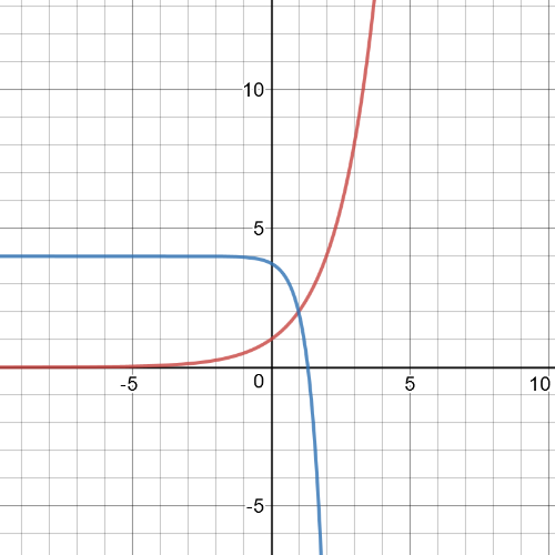
$textbf{The parent function:}$
$D=Bbb{R}$
$R=left(0,infty right)$
This function is $textbf{increasing}$ on $left(0,infty right)$ and have $textbf{horizontal asymptote}$ defined by $y=0$.
$textbf{Transformed function:}$
$D=Bbb{R}$
$R=left(-infty,2 right)$
This function is $textbf{decreasing}$ on $left(-infty,2 right)$ and have a $textbf{horizontal asymptote}$ defined by $y=4$.
#### (c)
$y=-2f(3(x-1))+4=-2cdot2^{3(x-1)}+4=-2^{3(x-1)+1}+4=-2^{3x-2}+4$
Here we have $textbf{vertical strech}$ by a factor of 3 and $textbf{translation}$ for 2 units to the right. So, the transformation of coordinates is:
$left(x,y right)rightarrowleft(x+2,3y right)$
$Rightarrow$ $left(1,8 right)rightarrowleft(3,24 right)$
#### (b)
Here we have $textbf{horizontal compression}$ by a factor of $dfrac{1}{2}$ and $textbf{translation}$ for 1 unit to the left and for 4 units down. So, the transformation of coordinates is:
$left(x,y right)rightarrowleft(dfrac{1}{2}x-1,y-4 right)$
$Rightarrow$ $left(1,8 right)rightarrowleft(-dfrac{1}{2},4 right)$
#### (c)
Here we have $textbf{horizontal compression}$ by -1, $textbf{vertical strech}$ by a factor of -2 and $textbf{translation}$ 7 units down. So, the transformation of coordinates is:
$left(x,y right)rightarrowleft(-x,-2y-7 right)$
$Rightarrow$ $left(1,8 right)rightarrowleft(-1,-23 right)$
#### (d)
Here we have $textbf{horizontal strech}$ by $dfrac{1}{4}$ and $textbf{vertical strech}$ by a factor of -1 and $textbf{translation}$ for 1 unit to the left. So, the transformation of coordinates is:
$left(x,y right)rightarrowleft(dfrac{1}{4}x-1,-y right)$
$Rightarrow$ $left(1,8 right)rightarrowleft(-dfrac{3}{4},-8 right)$
Here we have $textbf{horizontal compression}$ by factor -1 and $textbf{vertical strech}$ by a factor of -1 and $textbf{translation}$. So, the transformation of coordinates is:
$left(x,y right)rightarrowleft(-x,-y right)$
$Rightarrow$ $left(1,8 right)rightarrowleft(-1,-8 right)$
#### (f)
Here we have $textbf{horizontal compression}$ by a factor of 2 and $textbf{vertical strech}$ by a factor of $dfrac{1}{2}$ and $textbf{translation}$ for 3 units to the left and 3 units up. So, the transformation of coordinates is:
$left(x,y right)rightarrowleft(2x-3,dfrac{1}{2}y+3 right)$
$Rightarrow$ $left(1,8 right)rightarrowleft(-1,7 right)$
$textbf{Transformed function}$ is $g(x)=sqrt{x-2}$
$D=left[2,infty right)$
$R=left[0,infty right)$
#### (b)
$textbf{Transformed function}$ is $h(x)=2sqrt{x-1}+4$
$D=left[1,infty right)$
$R=left[4,infty right)$
#### (c)
$textbf{Transformed function}$ is $k(x)=sqrt{-x}+1$
$D=left(-infty,0 right]$
$R=left[1,infty right)$
#### (d)
$textbf{Transformed function}$ is $j(x)=3sqrt{2(x-5)}-3$
$D=left[5,infty right)$
$R=left[-3,infty right)$
First transformed function, $y=5x^2-3$ has $textbf{horizontal comression}$ by $dfrac{1}{5}$ and $textbf{translation}$ 3 units down.
The second transformed function is $y=5(x^2-3)$, it has $textbf{vertical strech}$ by a factor of 5 and $textbf{translation}$ 3 units on the right.
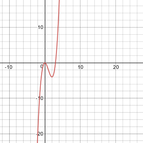
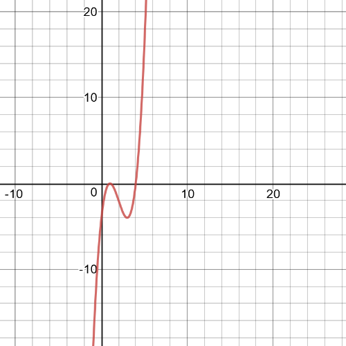
$f$ is $textbf{increasing}$ on intervals $left(-infty,0 right]$ and on $left[2,infty right)$ and it is $textbf{decreasing}$ on interval $left(0,2 right)$
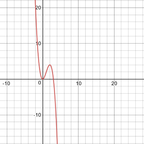
$h$ is $textbf{decreasing}$ on intervals $left(-infty,0 right]$ and on $left[2,infty right)$ and it is $textbf{increasing}$ on interval $left(0,2 right)$
Now, we are comparing functions $f$ and $g$:
$g$ has the same properties as function $f$ except that graph of $g$ is $textbf{translated}$ 1 unit to the right.
Here we have $textbf{vertically strech}$ by a factor of 4.
#### (b)
Here we have $textbf{horizontall compression}$ by $dfrac{1}{2}$
#### (c)
Here we are prooving that those two functions are the same functions:
$y=(2x)^2=2^2x^2=4x^2$
So, they are really the same functions.
$y=2f(x+1)-4$.
So, according to this, we have following $textbf{transformation of coordinates}$:
$left(x,y right)rightarrowleft(x-1,2y-4 right)$
We are given transformed coordinates, and that is point $left(4,5 right)$. In order to find the appropriate point on the parental function graph, the coordinates of the transfor- mated points must satisfy the following equations:
$x-1=3$ $wedge$ $2y-4=6$ $Rightarrow$ $x=4$ $wedge$ $y=5$
So, original point on the graph of $y=f(x)$ is $left(4,5 right)$.
left(4,5 right)
$$
Here we have $textbf{horizontal compression}$ by $dfrac{1}{3}$ and $textbf{translation}$ 2 units left.
#### (b)
Because, $textbf{algebraically}$, those functios are the same. Really:
$y=f(3(x+2))=f(3x+6)$
#### (c)
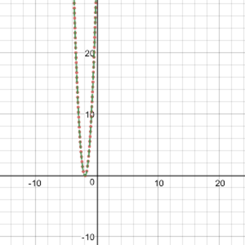
We have that our $textbf{parent function}$ in this case is $f(x)=x^2$.
First transformation of this function is: $y=f(3(x+2))=(3(x+2))^2$
Second transformation is: $y=f(3x+6)=(3x+6)^2$
Here we have the graphs of previous transformed functions, where that one with red dots is first transformation, and with green dots is second transformation. We can see from this graph that $textbf{they are the same transformed function}$.