#### (a)

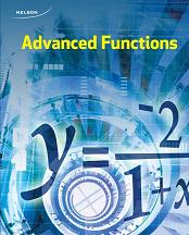
Use the graph to determine $f(2)$ and $f(7)$.

$f(2)=4$

$f(3)=1.5$

$y=dfrac{1.5-4}{7-2}=-0.5$

#### (b)

$textbf{The slope of the tangent line is}$ $-3$, we can see that from following gaph:

(a) $-0.5$; (b) $-3$

Use the difference quotient to help you estimate the average rate of change at $x=2$.Use $h=0.01$.

$dfrac{f(a+h)-f(a)}{h}=dfrac{f(2)-f(2.01)}{0.01}=dfrac{3.97-4}{0.01}=-3$

$textbf{So, the answers at $1.$ task and here match}$.

$-3$, it matches

On the following picture there is a graph of the given function.Have the calculator draw a line tangent to point $x=2$.We can see that the slope is $-3$, so, $textbf{the instaneous rate of change at}$ $x=2$ is $-3$.

$-3$

Use the difference quotient to determine the instaneous rate of change of $f(x)=dfrac{x}{x-1}$ at $(2,-1)$.The difference quotient is:

$f(x)=dfrac{f(a+h)-f(a)}{h}$, we can use $h=0.01$.

$f(2.01)=dfrac{2.01}{2.01-4}=-1.01$

$textbf{Difference quotient}$ = $dfrac{-1.01-(-1)}{0.01}=-1$

$-1$

Use the difference quotient to determine the instaneous rate of change for each functin.The difference quotient is $f(x)=dfrac{f(a+h)-f(a)}{h}$, we can take $h=0.01$.
#### (a)

$y=dfrac{1}{25-x}, x=13$

$f(13)=dfrac{1}{25-13}=dfrac{1}{12}$

$f(13.01)=dfrac{1}{25-13.01}=dfrac{1}{11.999}$

$textbf{Difference Quotient}$ = $dfrac{dfrac{1}{11.99}-dfrac{1}{12}}{0.001}=0.01$
#### (b)

$y=dfrac{17x+3}{x^2+6}, x=-5$

$f(-5)=dfrac{17(-5)+3}{(-5)^2+6}=-2.645$

$f(-4.99)=dfrac{17(-4.99)+3}{(-4.99)^2+6}=-2.648$

$textbf{Difference Quotient}$ = $dfrac{-2.648-(-2.645)}{0.01}=-dfrac{0.003}{0.01}=-0.3$
#### (c)

$y=dfrac{x+3}{x-2}, x=4$

$f(4)=dfrac{4+3}{4-2}=3.5$

$f(4.01)=dfrac{4.01+3}{4.01-2}=3.487$

$textbf{Difference Quotient}$ = $dfrac{3.487-3.5}{0.01}=-dfrac{0.013}{0.01}=-1.3$

#### (d)

$y=dfrac{-3x^2+5x+6}{x+6}, x=-3$

$f(-3)=dfrac{-3(-3)^2+5(-3)+6}{-3+6}=6$

$f(-3.01)=dfrac{-3(-3.01)^2+5(-3.01)+6}{-3.01+6}=6.06$

$textbf{Difference Quotient}$ = $dfrac{6.06-6}{0.01}=-dfrac{0.06}{0.01}=6$

(a) $0.01$; (b) $-0.3$; (c) $-1.3$; (d) $6$

Use the difference quotient to determine the instantaneous rate of change for each function. The difference quotient is $f(x)=dfrac{f(a+h)-f(a)}{h}$. Use $0.01$ for $h$. The point where there is no tangent line would be any vertical asymptotes.

#### (a)

$f(x)=dfrac{-5x}{2x+3}, x=2$

$f(2)=dfrac{-5(2)}{2(2)+3} = dfrac{-10}{7}= -1.429$

$f(2.01)=dfrac{-5(2.01)}{2(2.01)+3}= -1.432$

$textbf{Difference Quotient}$ = $dfrac{1.432-(-1.429)}{0.01}=286.1$

$textbf{The vertical asymptote would occur at $x= -1.5$}$.
#### (b)

$f(x)=dfrac{x-6}{x+5}, x= -7$

$f(-7) = dfrac{(-7)-6}{(-7)+5}=dfrac{-13}{-2}= 6.5$

$f(-7.01)=dfrac{(-7.01)-6}{(-7.01)+5}= dfrac{-13.01}{-2.01}= 6.4726$

$textbf{Difference Quotient}$ = $dfrac{6.4726-6.5}{0.01}= -2.74$

$textbf{The vertical asymptote would occur at}$ $x = -5$

#### (c)

$f(x)=dfrac{2x^2-6x}{3x+5}, x= -2$

$f(-2)=dfrac{2(-2)^2-6(-2.01)}{3(-2)+5}= -20$

$f(-2.01)=dfrac{2(-2.01)^2-6(-2.01)}{3(-2.01)+5}= -19.5535$

$textbf{Difference Quotient}$= $dfrac{-19.5535-(-20)}{0.01}= 44.65$

$textbf{The vertical asymptote would occur at}$ $x= -dfrac{5}{3}$

#### (d)

$f(x)=dfrac{5}{x-6}, x= 4$

$f(4)=dfrac{5}{(4)-6}=-2.5$

$f(4.01)=dfrac{5}{(4.01)-6}= -2.5126$

$textbf{Difference Quotient}$ = $dfrac{-2.5126-(-2.5)}{0.01}= -1.26$

$textbf{The vertical asymptotet occurs at $x=6$}$.

(a) $x= -1.5$
(b) $x = -5$
(c) $x= -dfrac{5}{3}$
(d) $x=6$

The function that models the concentration of the pollutant in the water is $c(t)=dfrac{27t}{10000+3t}$, where the units of $t$ are minutes.
#### (a)

There are $60$ minutes in $1$ hour, so, find $c(60)$:

$c(60)=dfrac{27cdot60}{10000+3cdotcdot60}=0.1591$

$c(60.01)=dfrac{27cdot60.01}{10000+3cdot60.01}=0.1592$

$textbf{Difference Quotient}$ = $dfrac{0.1592-0.1591}{0.01}=0.01$.
#### (b)

There are 10080 minutes in one week, so, determine c(10080):

$c(10080)=dfrac{27cdot10080}{10000+3cdotcdot10080}=6.76$

$c(10080.01)=dfrac{27cdot10080.01}{10000+3cdot10080.01}=6.7634$

$textbf{Difference Quotient}$ = $dfrac{6.7634-6.76}{0.01}=0.34$.

(a) $0.01$; (b) $0.34$

#### (a)

The demand function is $f(x)=dfrac{15x}{2x^2+11x+5}$.This function tells you

the price of the cakes for every $1000$ cakes.The revenue function would be the number of cakes sold, $x$, times the price of cakes for that number of cakes sold $dfrac{15x}{2x^2+11x+5}$.So, $textbf{the revenue function}$ is $p(x)=dfrac{15x}{2x^2+11x+5}$.
#### (b)

Use the difference quotient to determine the marginal revenue for $x=0.75$ and $x=2$.

$f(x)=dfrac{15x}{2x^2+11x+5}$

$f(0.75)=dfrac{15cdot0.75}{2(0.75)^2+11cdot0.75+5}=0.7826$

$f(0.751)=dfrac{15cdot0.751}{2(0.751)^2+11cdot0.751+5}=0.7829$

$textbf{Difference Quotient}$ = $dfrac{0.7829-0.7826}{0.001}=0.3$

$textbf{The marginal revenue at $x=0.75$ is $0.3$}$

Now, find the marginal revenue for $x=2$:

$f(2)=dfrac{15cdot2}{2cdot2^2+11cdot2+5}=0.8571$

$f(2.01)=dfrac{15cdot2.01}{2cdot2.01^2+11cdot2.01+5}=0.8568$

$textbf{Difference Quotient}$ = $dfrac{0.8568-0.8571}{0.01}=-0.03$

$textbf{The marginal revenue at $x=2$ is $-0.03$}$

(a) $p(x)=dfrac{15x}{2x^2+11x+5}$;

(b) The marginal revenue at $x=0.75$ is $0.3$, the marginal revenue at $x=2$ is $-0.03$

#### (a)

Since $x$ is measured in thousands, find $C(3)$.

The function is $C(x)=dfrac{x^2-4x+20}{x}$

$C(3)=dfrac{3^2+4cdot3+4cdot3+20}{3}=5.67$

$$
textbf{The average cost per T-shirt is $5.76$$ .}
$$

#### (b)

Determine $C(3.01)$ and use this value in the difference quotient to help you estimate the average rate of change of the average price of a T-shirt when the factory is producing $3000$ of them.

$C(3.01)=dfrac{3.01^2+4cdot3.01+4cdot3+20}{3.01}=5.65$

$textbf{Difference Quotient}$ = $dfrac{5.65-5.67}{0.01}=-2$

(a) $5.67$; (b) $-2$

The function is $N(t)=dfrac{100t^3}{100+t^3}$.

#### (a)

$N(6)=dfrac{100(6)^3}{100+(6)^3}=dfrac{21600}{316}=68.35$

$N(6.01)=dfrac{100(6.01)^3}{100+(6.01)^3}=dfrac{21708.18}{317.08}=68.46$

$textbf{Difference Quotient}$=$dfrac{68.46-68.35}{0.01}=-11$

#### (b)

$N(12)=dfrac{100(12)^3}{100+(12)^3}=dfrac{172800}{1828}=94.53$

$N(12.01)=dfrac{100(12.01)^3}{100+(12.01)^3}=dfrac{173232.36}{1832.32}=94.54$

$textbf{Difference Quotient}$=$dfrac{94.54-94.53}{0.01}=1$

#### (c)

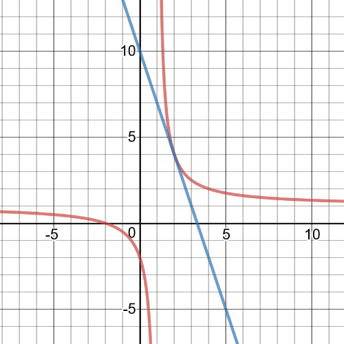
The number of houses that were built increases slowly at first, but rises rapidly between the third and sixth months. During the last six months, the rate at which the houses were built decreases.On the following picture there is a $textbf{graph}$ of given function:

(a)$-11$

(b)$1$

(c) see solution

Examine the interval $14leq xleq15$.Find the rate of change over the interval.

$f(15)=dfrac{15-2}{15-5}=dfrac{13}{10}=1.3$

$f(14)=dfrac{14-2}{14-5}=dfrac{12}{9}=1.33$

$dfrac{1.3-1.33}{15-14}= -0.03$

The slope over the interval $14leq x leq15$ is $m=-0.03$,which is approximately $0$. Now find the instantaneous rate of change at $14.5$.

$f(14.5)=dfrac{14.5-2}{14.5-5}=dfrac{12.5}{9.5}=1.316$

$f(14.51)=dfrac{14.51-2}{14.51-5}=dfrac{12.51}{9.51}=1.315$

$dfrac{1.315-1.316}{14.51-14.5}= -0.1$

The instantaneous rate of change at the point $14.5$ is $-0.01$, which is approximately $0$. The rate of change over the interval and at the specific point is about $0$.

$14leq x leq15$ is $m=-0.03$

$14.5$ is $-0.01$

#### (a)

I would find $s(0)$ and $s(6)$ and would then solve $dfrac{s(6)-s(0)}{6-0}$.

#### (b)

The average rate of change over this interval gives the object’s speed.

#### (c)

To find the instantaneous rate of change at a specific point, you could find the slope of the line that is tangent to the function $s(t)$ at the specific point. $textbf{You could also find the average rate of change on either side of the point for smaller and smaller intervals until it stabilizes to a constant.}$ It is generaly eaiser to find the instantaneous rate using a graph, but the second method is more accurate.

#### (d)

The instantaneous rate of change for a specific time $t$,is the acceleration of the object at this time.

On the following picture there is $textbf{a graph}$ of function $f(x)=dfrac{4x}{x^2+1}$:

Find $x=-sqrt{3}$ on the graph and use the calculator to find the line tangent to the graph at this point.

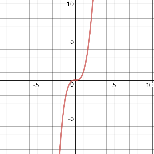
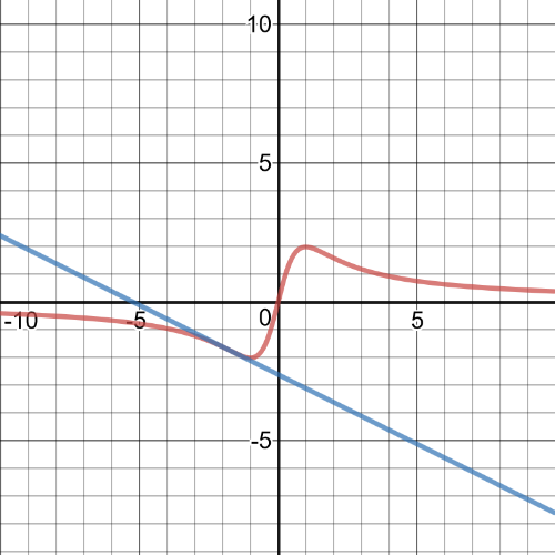
$textbf{The equation of the line tangent to the function at $(-sqrt{3},-sqrt{3})$ is}$ $y=-0.5x-2.598$.

On the following picture is graph of the function and tangent line at the point $(-sqrt{3},-sqrt{3})$

$textbf{The equation of the line tangent to the function at $(sqrt{3},sqrt{3})$ is $y=-0.5x+2.598$}$.

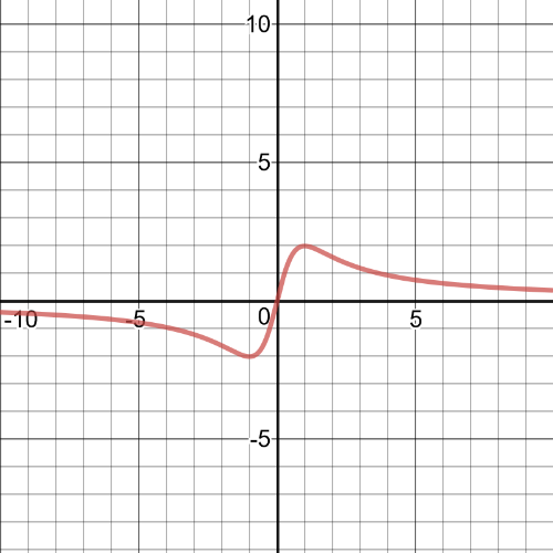
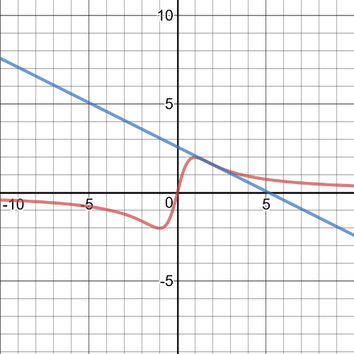
On the following picture there is a graph of the function and tangent line.

$textbf{The equation of the line tangent to the function at $(0,0)$ is $y=4x$}$.

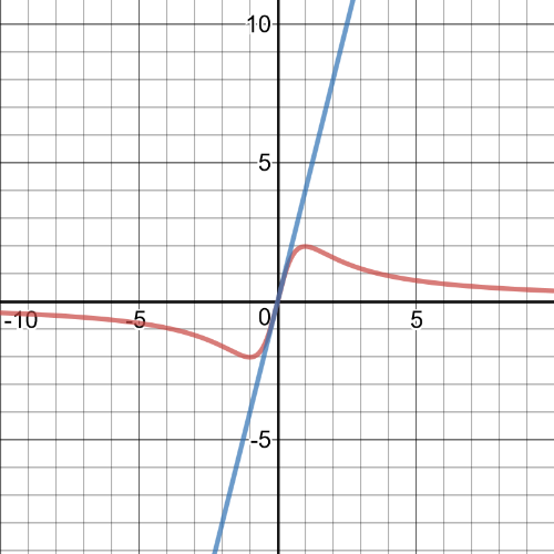
On the following picture there is a graph of the function and tangent line at point $(0,0)$.

$(-sqrt{3},-sqrt{3})$ – $y=-0.5x-2.598$;

$(sqrt{3},sqrt{3})$ – $y=-0.5x+2.598$;

$(0,0)$ – $y=4x$.

Examine the graph of the function. Use your calculator to zoom into points around the origin. The graph appears to be a straight line at this point, and so the instantaneous rates of change at $(0,0)$ will likely be pretty close to the instantaneous rate of change at $(0,0)$, which is $4$.Because the graph is almost a straight line at $(0,0)$ the rate of change is neither increasing nor decreasing; it will remain constant. Therefore the rate of change at this rate of change will be $0$.